


知识点:
1. 不平衡数据集的处理策略:过采样、修改权重、修改阈值
2. 交叉验证代码
作业:
从示例代码可以看到 效果没有变好,所以很多步骤都是理想是好的,但是现实并不一定可以变好。这个实验仍然有改进空间,如下。
1. 我还没做smote+过采样+修改权重的组合策略,有可能一起做会变好。
2. 我还没有调参,有可能调参后再取上述策略可能会变好
针对上面这2个探索路径,继续尝试下去,看看是否符合猜测。
步骤一:数据预处理
# 先运行之前预处理好的代码
import pandas as pd
import pandas as pd    #用于数据处理和分析,可处理表格数据。
import numpy as np     #用于数值计算,提供了高效的数组操作。
import matplotlib.pyplot as plt    #用于绘制各种类型的图表
import seaborn as sns   #基于matplotlib的高级绘图库,能绘制更美观的统计图形。
import warnings
warnings.filterwarnings("ignore")

 # 设置中文字体(解决中文显示问题)
plt.rcParams['font.sans-serif'] = ['SimHei']  # Windows系统常用黑体字体
plt.rcParams['axes.unicode_minus'] = False    # 正常显示负号
data = pd.read_csv('data.csv')    #读取数据


# 先筛选字符串变量
discrete_features = data.select_dtypes(include=['object']).columns.tolist()
# Home Ownership 标签编码
home_ownership_mapping = {
    'Own Home': 1,
    'Rent': 2,
    'Have Mortgage': 3,
    'Home Mortgage': 4
}
data['Home Ownership'] = data['Home Ownership'].map(home_ownership_mapping)

# Years in current job 标签编码
years_in_job_mapping = {
    '< 1 year': 1,
    '1 year': 2,
    '2 years': 3,
    '3 years': 4,
    '4 years': 5,
    '5 years': 6,
    '6 years': 7,
    '7 years': 8,
    '8 years': 9,
    '9 years': 10,
    '10+ years': 11
}
data['Years in current job'] = data['Years in current job'].map(years_in_job_mapping)

# Purpose 独热编码,记得需要将bool类型转换为数值
data = pd.get_dummies(data, columns=['Purpose'])
data2 = pd.read_csv("data.csv") # 重新读取数据,用来做列名对比
list_final = [] # 新建一个空列表,用于存放独热编码后新增的特征名
for i in data.columns:
    if i not in data2.columns:
       list_final.append(i) # 这里打印出来的就是独热编码后的特征名
for i in list_final:
    data[i] = data[i].astype(int) # 这里的i就是独热编码后的特征名


# Term 0 - 1 映射
term_mapping = {
    'Short Term': 0,
    'Long Term': 1
}
data['Term'] = data['Term'].map(term_mapping)
data.rename(columns={'Term': 'Long Term'}, inplace=True) # 重命名列
continuous_features = data.select_dtypes(include=['int64', 'float64']).columns.tolist()  #把筛选出来的列名转换成列表

 # 连续特征用中位数补全
for feature in continuous_features:
    mode_value = data[feature].mode()[0]            #获取该列的众数。
    data[feature].fillna(mode_value, inplace=True)          #用众数填充该列的缺失值,inplace=True表示直接在原数据上修改。

# 最开始也说了 很多调参函数自带交叉验证,甚至是必选的参数,你如果想要不交叉反而实现起来会麻烦很多
# 所以这里我们还是只划分一次数据集
from sklearn.model_selection import train_test_split
X = data.drop(['Credit Default'], axis=1)  # 特征,axis=1表示按列删除
y = data['Credit Default'] # 标签
# 按照8:2划分训练集和测试集
X_train, X_test, y_train, y_test = train_test_split(X, y, test_size=0.2, random_state=42)  # 80%训练集,20%测试集
步骤二:基准模型作为参照
输入:
from sklearn.ensemble import RandomForestClassifier #随机森林分类器
from sklearn.metrics import accuracy_score, precision_score, recall_score, f1_score # 用于评估分类器性能的指标
from sklearn.metrics import classification_report, confusion_matrix #用于生成分类报告和混淆矩阵
import warnings #用于忽略警告信息
warnings.filterwarnings("ignore") # 忽略所有警告信息
# --- 1. 默认参数的随机森林 ---
# 评估基准模型,这里确实不需要验证集
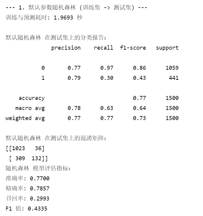
print("--- 1. 默认参数随机森林 (训练集 -> 测试集) ---")
import time # 这里介绍一个新的库,time库,主要用于时间相关的操作,因为调参需要很长时间,记录下会帮助后人知道大概的时长
start_time = time.time() # 记录开始时间
rf_model = RandomForestClassifier(random_state=42)
rf_model.fit(X_train, y_train) # 在训练集上训练
rf_pred = rf_model.predict(X_test) # 在测试集上预测
end_time = time.time() # 记录结束时间
print(f"训练与预测耗时: {end_time - start_time:.4f} 秒")
print("\n默认随机森林 在测试集上的分类报告:")
print(classification_report(y_test, rf_pred))
print("默认随机森林 在测试集上的混淆矩阵:")
print(confusion_matrix(y_test, rf_pred))
rf_accuracy = accuracy_score(y_test, rf_pred)
rf_precision = precision_score(y_test, rf_pred)
rf_recall = recall_score(y_test, rf_pred)
rf_f1 = f1_score(y_test, rf_pred)
print("随机森林 模型评估指标:")
print(f"准确率: {rf_accuracy:.4f}")
print(f"精确率: {rf_precision:.4f}")
print(f"召回率: {rf_recall:.4f}")
print(f"F1 值: {rf_f1:.4f}")输出:
步骤三:SMOTE过采样+权重调整的组合策略
输入:
# 1. SMOTE过采样+权重调整的组合策略
from imblearn.over_sampling import SMOTE
from imblearn.pipeline import Pipeline
from sklearn.model_selection import GridSearchCV
# 计算类别权重
minority_class = np.argmin(np.bincount(y_train))
majority_class = np.argmax(np.bincount(y_train))
scale_pos_weight = np.bincount(y_train)[majority_class] / np.bincount(y_train)[minority_class]
# 创建SMOTE和随机森林的pipeline
pipeline = Pipeline([
('smote', SMOTE(random_state=42)),
('rf', RandomForestClassifier(random_state=42, class_weight='balanced'))
])
# 训练模型
pipeline.fit(X_train, y_train)
# 2. 调参后再应用组合策略
# 定义参数网格
param_grid = {
'rf__n_estimators': [100, 200],
'rf__max_depth': [None, 10, 20],
'rf__min_samples_split': [2, 5],
'rf__min_samples_leaf': [1, 2]
}
# 使用F1分数作为评估指标(更适合不平衡数据)
scorer = make_scorer(f1_score, pos_label=minority_class)
# 创建网格搜索对象
grid_search = GridSearchCV(
estimator=pipeline,
param_grid=param_grid,
scoring=scorer,
cv=5,
n_jobs=-1
)
# 执行网格搜索
grid_search.fit(X_train, y_train)
# 输出最佳参数
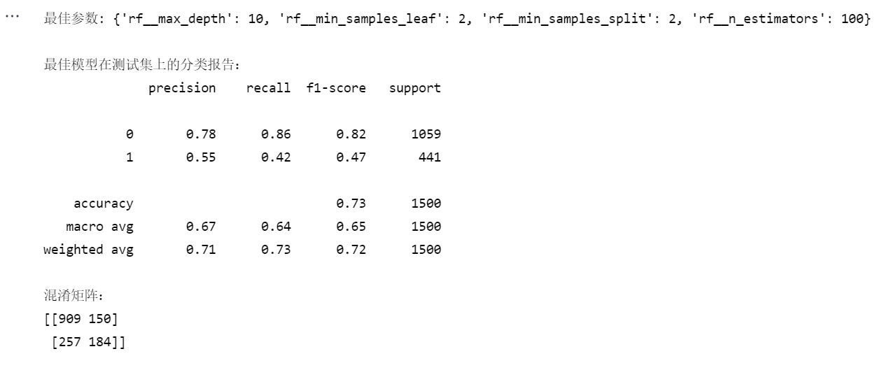
print("最佳参数:", grid_search.best_params_)
# 使用最佳参数训练最终模型
best_model = grid_search.best_estimator_
best_model.fit(X_train, y_train)
# 评估模型
y_pred = best_model.predict(X_test)
print("\n最佳模型在测试集上的分类报告:")
print(classification_report(y_test, y_pred))
print("混淆矩阵:")
print(confusion_matrix(y_test, y_pred))输出:
笔记
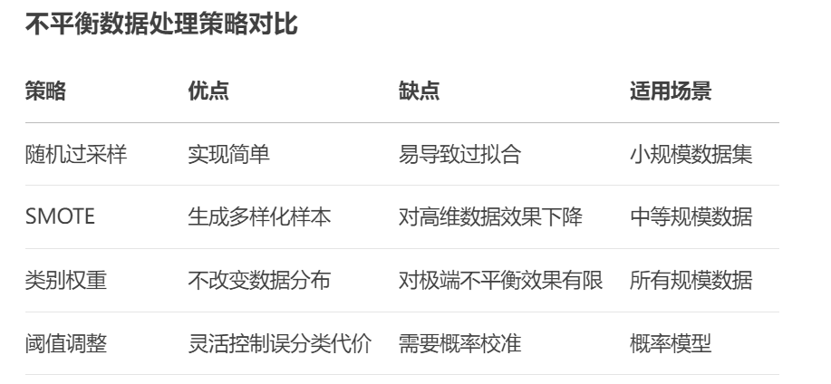
一、不平衡数据集处理策略
1. 过采样技术
1.1 随机过采样 (Random Oversampling)
from imblearn.over_sampling import RandomOverSampler

ros = RandomOverSampler(sampling_strategy='auto', random_state=42)
X_resampled, y_resampled = ros.fit_resample(X_train, y_train)

# 查看采样后分布
print("过采样后类别分布:", pd.Series(y_resampled).value_counts())特点:
-
简单复制少数类样本
-
可能导致过拟合
-
适合小规模数据集
1.2 SMOTE (Synthetic Minority Oversampling Technique)
from imblearn.over_sampling import SMOTE

smote = SMOTE(sampling_strategy=0.5,  # 使少数类达到多数类的50%
              k_neighbors=5,
              random_state=42)
X_smote, y_smote = smote.fit_resample(X_train, y_train)特点:
-
通过插值生成新样本
-
比随机过采样更不易过拟合
-
参数
k_neighbors影响生成样本质量
1.3 ADASYN (Adaptive Synthetic Sampling)
from imblearn.over_sampling import ADASYN

adasyn = ADASYN(sampling_strategy='minority',
                n_neighbors=5,
                random_state=42)
X_adasyn, y_adasyn = adasyn.fit_resample(X_train, y_train)特点:
-
根据样本密度自适应生成样本
-
对难分类样本生成更多合成样本
-
计算成本高于SMOTE
2. 类别权重调整
2.1 自动计算类别权重
from sklearn.utils.class_weight import compute_class_weight

classes = np.unique(y_train)
weights = compute_class_weight('balanced', classes=classes, y=y_train)
class_weights = dict(zip(classes, weights))

# 在模型中使用
model = RandomForestClassifier(class_weight=class_weights, random_state=42)
2.2 自定义权重
# 根据业务需求设置权重
custom_weights = {0: 1, 1: 3}  # 少数类(1)的误分类代价是多数类(0)的3倍
model = RandomForestClassifier(class_weight=custom_weights, random_state=42)权重设置原则:
-
少数类样本的误分类代价越高,权重应越大
-
可通过网格搜索寻找最优权重比
3. 阈值调整 (Threshold Moving)
3.1 基于概率调整决策阈值
from sklearn.metrics import precision_recall_curve

# 获取预测概率
y_probs = model.predict_proba(X_test)[:, 1]

# 计算最佳阈值
precision, recall, thresholds = precision_recall_curve(y_test, y_probs)
f1_scores = 2 * (precision * recall) / (precision + recall)
optimal_threshold = thresholds[np.argmax(f1_scores)]

# 应用新阈值
y_pred_adj = (y_probs >= optimal_threshold).astype(int)
3.2 代价敏感学习
from sklearn.metrics import make_scorer
from sklearn.metrics import confusion_matrix

def cost_sensitive_score(y_true, y_pred):
    tn, fp, fn, tp = confusion_matrix(y_true, y_pred).ravel()
    cost = fp * 1 + fn * 5  # 假设假阴性的代价是假阳性的5倍
    return -cost  # 返回负代价以便最大化

cost_scorer = make_scorer(cost_sensitive_score, greater_is_better=False)
二、交叉验证实现
1. 基础交叉验证
1.1 K折交叉验证
from sklearn.model_selection import cross_val_score
from sklearn.metrics import make_scorer
from sklearn.metrics import f1_score

# 使用f1加权平均作为评估指标
f1_scorer = make_scorer(f1_score, average='weighted')

scores = cross_val_score(
    estimator=model,
    X=X_train,
    y=y_train,
    cv=5,  # 5折交叉验证
    scoring=f1_scorer,
    n_jobs=-1
)

print("交叉验证F1分数:", scores)
print("平均F1分数: {:.3f} ± {:.3f}".format(scores.mean(), scores.std()))
1.2 分层K折交叉验证
from imblearn.pipeline import make_pipeline
from sklearn.model_selection import StratifiedKFold

# 创建包含采样的流水线
pipeline = make_pipeline(
    SMOTE(random_state=42),
    RandomForestClassifier(random_state=42)
)

# 分层交叉验证
skf = StratifiedKFold(n_splits=5, shuffle=True, random_state=42)
scores = cross_val_score(pipeline, X_train, y_train, cv=skf, scoring=f1_scorer)适用场景:
-
分类问题
-
保持每折中类别比例与原数据一致
2. 不平衡数据的交叉验证
2.1 在交叉验证中应用采样
from imblearn.pipeline import make_pipeline
from sklearn.model_selection import StratifiedKFold

# 创建包含采样的流水线
pipeline = make_pipeline(
    SMOTE(random_state=42),
    RandomForestClassifier(random_state=42)
)

# 分层交叉验证
skf = StratifiedKFold(n_splits=5, shuffle=True, random_state=42)
scores = cross_val_score(pipeline, X_train, y_train, cv=skf, scoring=f1_scorer)注意事项:
-
采样只应在训练折叠上进行,验证折叠保持原始分布
-
使用
imblearn.pipeline确保采样步骤正确执行
2.2 重复交叉验证
from sklearn.model_selection import RepeatedStratifiedKFold

rskf = RepeatedStratifiedKFold(
    n_splits=5,
    n_repeats=3,  # 重复3次
    random_state=42
)
scores = cross_val_score(pipeline, X_train, y_train, cv=rskf, scoring=f1_scorer)优点:
-
更可靠的性能估计
-
减少因数据划分导致的方差
3. 时间序列交叉验证
from sklearn.model_selection import TimeSeriesSplit

tscv = TimeSeriesSplit(n_splits=5)
scores = cross_val_score(model, X_train, y_train, cv=tscv, scoring=f1_scorer)特点:
-
保持时间顺序
-
训练集总是早于测试集
-
适合时间相关数据
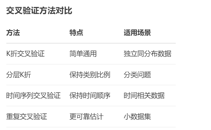
三、总结对比表


 被折叠的 条评论
为什么被折叠?
被折叠的 条评论
为什么被折叠?
 到【灌水乐园】发言


