代码
import numpy as np
import pandas as pd
import matplotlib.pyplot as plt


# 线性回归(多变量)
# 房价预测。 ex1data2.txt:面积、卧室数、房价

# 代价函数
def computeCost(X, Y, theta):
    inner = np.power((X * theta.T) - Y, 2)
    return np.sum(inner) / (2 * len(X))


# 梯度下降
def gradientDescent(X, Y, theta, alpha, iters):
    temp = np.matrix(np.zeros(theta.shape))
    parameters = int(theta.shape[1])
    cost = np.zeros(iters)

    for i in range(iters):
        error = X * theta.T - Y

        for j in range(parameters):
            term = np.multiply(error, X[:, j])
            temp[0, j] = temp[0, j] - alpha / len(X) * np.sum(term)

        theta = temp
        cost[i] = computeCost(X, Y, theta)

    return theta, cost


path = 'ex1data2.txt'
data = pd.read_csv(path, header=None, names=['Size', 'Bedrooms', 'Price'])
# print(data) #for checking

# 保存mean, std, mins, maxs, data
means = data.mean().values
stds = data.std().values
mins = data.min().values
maxs = data.max().values
data_ = data.values
data.describe()
# des = data.describe()
# print(des)
# 计算了数据集data中每一列的均值(mean)、标准差(std)、最小值(min)和最大值(max),
# 分别保存在means、stds、mins和maxs这四个变量中。
# 然后,将整个数据集转换为NumPy数组,并保存在data_变量中
# 调用data.describe()方法会生成关于数据集data的描述性统计信息,包括计数、均值、标准差、最小值、25th、50th和75th百分位数以及最大值

# 特征缩放
data = (data - data.mean()) / data.std()  # 对数据集data进行标准化操作#建议看课后理解
data.head()  # data.head()方法会显示标准化后的数据集的前几行,以便查看标准化后的数据情况

# add ones column
data.insert(0, 'Ones', 1)

# set X(training data) and Y(target variable)
cols = data.shape[1]
X = data.iloc[:, :cols - 1]
Y = data.iloc[:, cols - 1:cols]

# convert to matrices and initialize theta
X = np.matrix(X.values)
Y = np.matrix(Y.values)
theta = np.matrix(np.array([0, 0, 0]))

# perform linear regression on the data set
alpha = 0.01
iters = 1000
g, cost = gradientDescent(X, Y, theta, alpha, iters)

# get the cost(error) of the model
computeCost(X, Y, g)
# print(g) # what we get is matrix

# 画出cost图像
fig, ax = plt.subplots(figsize=(12, 8))
ax.plot(np.arange(iters), cost, 'r')
ax.set_xlabel('Iterations')
ax.set_ylabel('Cost')
ax.set_title('Error vs Training Epoch')
plt.show()  # 很显然,比one——variable效果好的多


# 参数转化为缩放前
def theta_transform(theta, means, stds):
    temp = means[:-1] * theta[1:] / stds[:-1]
    theta[0] = (theta[0] - np.sum(temp)) * stds[-1] + means[-1]
    theta[1:] = theta[1:] * stds[-1] / stds[:-1]
    return theta.reshape(1, -1)


g_ = np.array(g.reshape(-1, 1))
means = means.reshape(-1, 1)
stds = stds.reshape(-1, 1)
transform_g = theta_transform(g_, means, stds)


#  print(transform_g)

# 预测价格
def predictPrice(x, y, theta):
    return theta[0, 0] + theta[0, 1] * x + theta[0, 2] * y


# 2104, 3, 399900,
price = predictPrice(2104, 3, transform_g)
# print(price)


# 画出拟合平面 the old version
from mpl_toolkits.mplot3d import Axes3D

fig = plt.figure()
ax = Axes3D(fig)  # 这为吴恩达原代码
# 若想要不出warninig,可讲上行改为: ax = fig.add_subplot(111, projection='3d')  # 使用add_subplot添加子图,并指定投影为3D
X_ = np.arange(mins[0], maxs[0] + 1, 1)
Y_ = np.arange(mins[1], maxs[1] + 1, 1)
X_, Y_ = np.meshgrid(X_, Y_)
Z_ = transform_g[0, 0] + transform_g[0, 1] * X_ + transform_g[0, 2] * Y_

# 手动设置角度
ax.view_init(elev=25, azim=125)  # 可以自行更改角度来查看:(elev=10, azim=80) is a good choice

ax.set_xlabel('Size')
ax.set_ylabel('Bedrooms')
ax.set_zlabel('Price')

ax.plot_surface(X_, Y_, Z_, rstride=1, cstride=1, color='red')

ax.scatter(data_[:, 0], data_[:, 1], data_[:, 2])
plt.show()
# print(data2_, data2_.shape, type(data2_))


# second way which is the new one to solve this problem
# # 画出拟合平面
# from mpl_toolkits.mplot3d import Axes3D
# fig = plt.figure()
# ax = fig.add_subplot(111, projection='3d')  # 使用add_subplot添加子图,并指定投影为3D
#
# X_ = np.arange(mins[0], maxs[0]+1, 1)
# Y_ = np.arange(mins[1], maxs[1]+1, 1)
# X_, Y_ = np.meshgrid(X_, Y_)
# Z_ = transform_g[0,0] + transform_g[0,1] * X_ + transform_g[0,2] * Y_
#
# # 手动设置角度
# ax.view_init(elev=25, azim=125)
#
# ax.set_xlabel('Size')
# ax.set_ylabel('Bedrooms')
# ax.set_zlabel('Price')
#
# surf = ax.plot_surface(X_, Y_, Z_, rstride=1, cstride=1, color='red')  # 使用plot_surface绘制曲面

# ax.scatter(data_[:, 0], data_[:, 1], data_[:, 2])  # 绘制散点图
# #这里使用了fig.add_subplot(111, projection='3d')来添加子图并指定投影为3D,同时使用plot_surface来绘制曲面
# plt.show()
图例
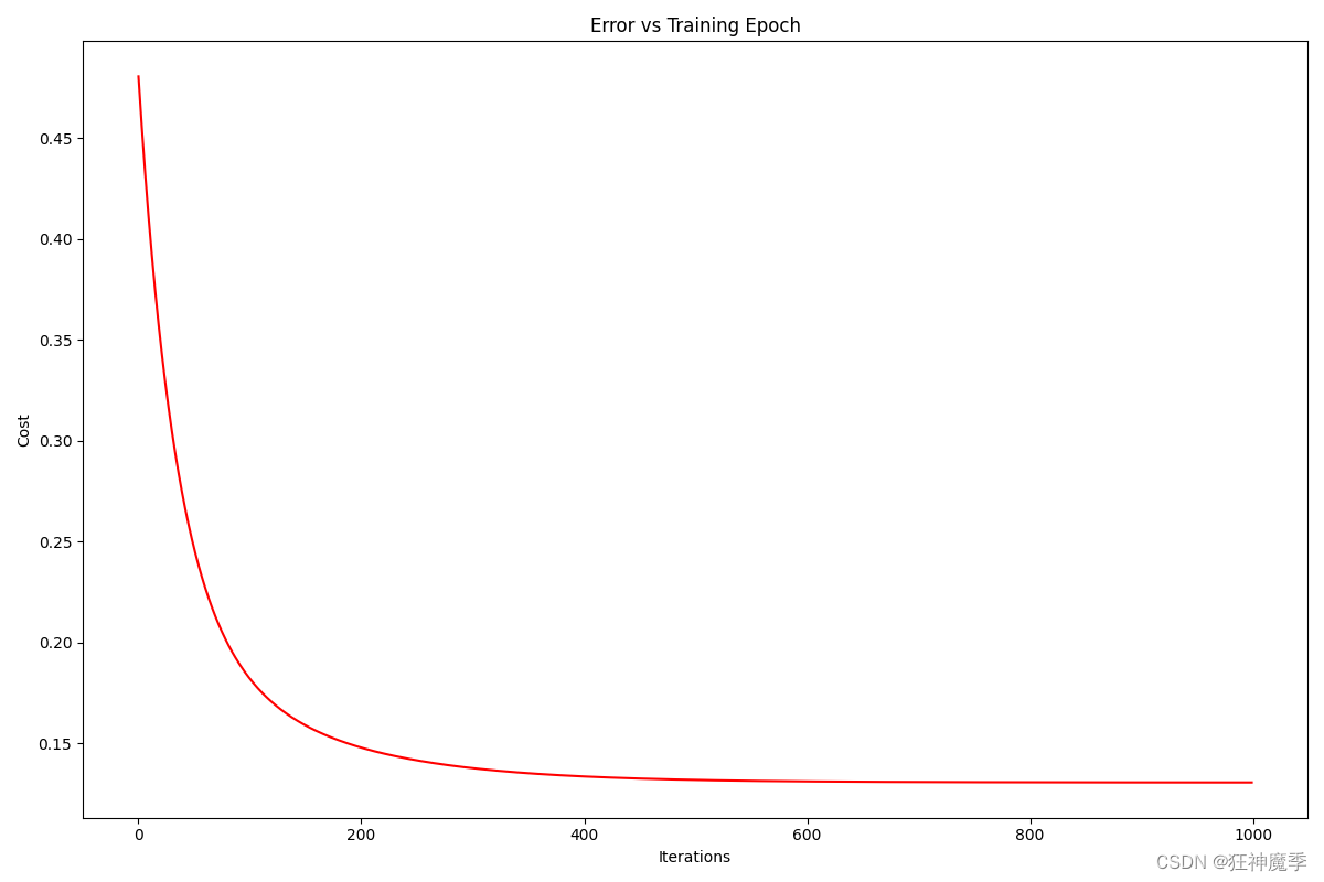
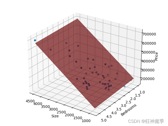


 本文介绍了使用Python进行线性回归模型的构建,包括数据预处理、代价函数计算、梯度下降优化算法,以及如何通过拟合平面可视化房价预测。作者详细展示了如何使用ex1data2.txt数据集进行房价预测,并展示了训练过程中的成本函数变化。


 被折叠的 条评论
为什么被折叠?
被折叠的 条评论
为什么被折叠?
 到【灌水乐园】发言


