


Practice Lab - Advice for Applying Machine Learning
In this lab, you will explore techniques to evaluate and improve your machine learning models.(应用机器学习的建议)
在本次实验中,您将探索评估和改善机器学习模型的技术。
Outline
- 1 - Packages
- 2 - Evaluating a Learning Algorithm (Polynomial Regression)(评估学习算法(多项式回归))
- 3 - Bias and Variance(偏差和方差)<img align=“Right”

- 4 - Evaluating a Learning Algorithm (Neural Network)(评估学习算法(神经网络))
- 5 - Model Complexity(复杂模型)
- 6 - Regularization(复杂模型添加正则化)
- 7 - Iterate to find optimal regularization value(迭代找到最优的正则化系数)
1 - Packages
First, let’s run the cell below to import all the packages that you will need during this assignment.
首先,运行下面的单元格导入所有你在这个作业中需要用到的包。
- numpy is the fundamental package for scientific computing Python.
- matplotlib is a popular library to plot graphs in Python.
- scikitlearn is a basic library for data mining
- tensorflow a popular platform for machine learning.
import numpy as np
%matplotlib widget
import matplotlib.pyplot as plt
from sklearn.linear_model import LinearRegression, Ridge,RidgeCV
from sklearn.preprocessing import StandardScaler, PolynomialFeatures
from sklearn.model_selection import train_test_split
from sklearn.metrics import mean_squared_error
import tensorflow as tf
from tensorflow.keras.models import Sequential
from tensorflow.keras.layers import Dense
from tensorflow.keras.activations import relu,linear
from tensorflow.keras.losses import SparseCategoricalCrossentropy
from tensorflow.keras.optimizers import Adam

import logging
logging.getLogger("tensorflow").setLevel(logging.ERROR)

from public_tests_a1 import *

tf.keras.backend.set_floatx('float64')
from assigment_utils import *

tf.autograph.set_verbosity(0)
2 - Evaluating a Learning Algorithm (Polynomial Regression)(评估一个学习算法(多项式回归))

Let’s say you have created a machine learning model and you find it fits your training data very well. You’re done? Not quite. The goal of creating the model was to be able to predict values for
假设你创建了一个机器学习模型,你发现它非常适合你的训练数据。你完成了吗?不完全是。创建模型的目的是能够预测
new examples.
How can you test your model’s performance on new data before deploying it?
在部署新数据之前,如何在新数据上测试模型的性能?
The answer has two parts:
答案有两部分:
- Split your original data set into “Training” and “Test” sets.(将原始数据集分成"训练"和"测试"集)
- Use the training data to fit the parameters of the model(使用训练数据来拟合模型的参数)
- Use the test data to evaluate the model on new data(使用测试数据来评估模型在新数据上的性能)
- Develop an error function to evaluate your model(开发一个误差函数来评价你的模型).
2.1 Splitting your data set(分割你的数据集)
Lectures advised reserving 20-40% of your data set for testing. Let’s use an sklearn function train_test_split to perform the split. Double-check the shapes after running the following cell.
讲座建议保留20-40%的数据集用于测试。让我们使用一个sklearn函数train_test_split来执行分割。运行以下单元格后,请再次检查形状。
# Generate some data
X,y,x_ideal,y_ideal = gen_data(18, 2, 0.7)
print("X.shape", X.shape, "y.shape", y.shape)

#split the data using sklearn routine
X_train, X_test, y_train, y_test = train_test_split(X,y,test_size=0.33, random_state=1)
print("X_train.shape", X_train.shape, "y_train.shape", y_train.shape)
print("X_test.shape", X_test.shape, "y_test.shape", y_test.shape)
X.shape (18,) y.shape (18,)
X_train.shape (12,) y_train.shape (12,)
X_test.shape (6,) y_test.shape (6,)
2.1.1 Plot Train, Test sets(绘制训练集,测试集)
You can see below the data points that will be part of training (in red) are intermixed with those that the model is not trained on (test). This particular data set is a quadratic function with noise added. The “ideal” curve is shown for reference.
您可以在下面看到,将成为训练一部分的数据点(红色)与模型未训练的数据点(测试)混合在一起。这个特殊的数据集是一个加了噪声的二次函数。“理想”曲线为参考。
fig, ax = plt.subplots(1,1,figsize=(4,4))
ax.plot(x_ideal, y_ideal, "--", color = "orangered", label="y_ideal", lw=1)
ax.set_title("Training, Test",fontsize = 14)
ax.set_xlabel("x")
ax.set_ylabel("y")

ax.scatter(X_train, y_train, color = "red",           label="train")
ax.scatter(X_test, y_test,   color = dlc["dlblue"],   label="test")
ax.legend(loc='upper left')
plt.show()

2.2 Error calculation for model evaluation, linear regression(模型评估的误差计算,线性回归)
When evaluating a linear regression model, you average the squared error difference of the predicted values and the target values.
当评估线性回归模型时,将预测值和目标值差的平方和取平均值。
J test ( w , b ) = 1 2 m test ∑ i = 0 m test − 1 ( f w , b ( x test ( i ) ) − y test ( i ) ) 2 (1) J_\text{test}(\mathbf{w},b) = \frac{1}{2m_\text{test}}\sum_{i=0}^{m_\text{test}-1} ( f_{\mathbf{w},b}(\mathbf{x}^{(i)}_\text{test}) - y^{(i)}_\text{test} )^2 \tag{1} Jtest(w,b)=2mtest1i=0∑mtest−1(fw,b(xtest(i))−ytest(i))2(1)
Exercise 1
Below, create a function to evaluate the error on a data set for a linear regression model.
在下面,创建一个函数来评估线性回归模型在数据集上的误差。
# UNQ_C1
# GRADED CELL: eval_mse
def eval_mse(y, yhat):
    """
    Calculate the mean squared error on a data set.
    Args:
      y    : (ndarray  Shape (m,) or (m,1))  target value of each example
      yhat : (ndarray  Shape (m,) or (m,1))  predicted value of each example
    Returns:
      err: (scalar)
    """
    m = len(y)
    err = 0.0
    for i in range(m):
    ### START CODE HERE ###
      err += (yhat[i] - y[i])**2
    err = err / (2 * m)
    ### END CODE HERE ###

    return(err)
y_hat = np.array([2.4, 4.2])
y_tmp = np.array([2.3, 4.1])
eval_mse(y_hat, y_tmp)

# BEGIN UNIT TEST
test_eval_mse(eval_mse)
# END UNIT TEST
[92m All tests passed.
def eval_mse(y, yhat):
    """
    Calculate the mean squared error on a data set.
    Args:
      y    : (ndarray  Shape (m,) or (m,1))  target value of each example
      yhat : (ndarray  Shape (m,) or (m,1))  predicted value of each example
    Returns:
      err: (scalar)
    """
    m = len(y)
    err = 0.0
    for i in range(m):
        err_i  = ( (yhat[i] - y[i])**2 )
        err   += err_i
    err = err / (2*m)
    return(err)
2.3 Compare performance on training and test data(比较训练数据和测试数据的表现)
Let’s build a high degree polynomial model to minimize training error. This will use the linear_regression functions from sklearn. The code is in the imported utility file if you would like to see the details. The steps below are:
让我们建立一个高次多项式模型来最小化训练误差。这将使用来自’ sklearn '的线性回归函数。如果您想查看详细信息,代码位于导入的实用程序文件中。步骤如下:
- create and fit the model. (‘fit’ is another name for training or running gradient descent).(创建并拟合模型。(“fit”是训练或运行梯度下降的另一个名称))
- compute the error on the training data.(在训练数据上计算误差)
- compute the error on the test data.(在测试数据上计算误差)
# create a model in sklearn, train on training data
degree = 10
lmodel = lin_model(degree)
lmodel.fit(X_train, y_train)

# predict on training data, find training error
yhat = lmodel.predict(X_train)
err_train = lmodel.mse(y_train, yhat)

# predict on test data, find error
yhat = lmodel.predict(X_test)
err_test = lmodel.mse(y_test, yhat)
The computed error on the training set is substantially less than that of the test set.
训练集的计算误差基本上小于测试集的计算误差。
print(f"training err {err_train:0.2f}, test err {err_test:0.2f}")
training err 58.01, test err 171215.01
The following plot shows why this is. The model fits the training data very well. To do so, it has created a complex function. The test data was not part of the training and the model does a poor job of predicting on this data.
下面的图表显示了为什么这是如此。该模型很好地拟合了训练数据。为了做到这一点,它创建了一个复杂的函数。测试数据不是训练的一部分,模型在预测这些数据时做得不好。
This model would be described as 1) is overfitting, 2) has high variance 3) ‘generalizes’ poorly.
该模型将被描述为1)过拟合,2)具有高方差3)“概括”不佳。
# plot predictions over data range
x = np.linspace(0,int(X.max()),100)  # predict values for plot
y_pred = lmodel.predict(x).reshape(-1,1)

plt_train_test(X_train, y_train, X_test, y_test, x, y_pred, x_ideal, y_ideal, degree)

The test set error shows this model will not work well on new data. If you use the test error to guide improvements in the model, then the model will perform well on the test data… but the test data was meant to represent new data.
测试集误差显示,该模型在新数据上不会工作很好。如果您使用测试误差来指导模型改进,那么模型将在测试数据上表现良好…但测试数据旨在代表新数据。
You need yet another set of data to test new data performance.
你需要另一组数据来测试新数据性能。
The proposal made during lecture is to separate data into three groups. The distribution of training, cross-validation and test sets shown in the below table is a typical distribution, but can be varied depending on the amount of data available.
在讲座中提出的建议是将数据分为三个组。下表中显示的训练、交叉验证和测试集分布是典型的分布,但可以根据可用数据的数量而有所不同。
| data | % of total | Description |
|---|---|---|
| training(训练集) | 60 | Data used to tune model parameters w w w and b b b in training or fitting(在训练或拟合中用于调整模型参数 w w w和 b b b的数据) |
| cross-validation(交叉验证集) | 20 | Data used to tune other model parameters like degree of polynomial, regularization or the architecture of a neural network.(用于调整其他模型参数的数据,如多项式度、正则化或神经网络的架构。) |
| test(测试集) | 20 | Data used to test the model after tuning to gauge performance on new data(用于在调优后测试模型以衡量新数据上的性能的数据) |
Let’s generate three data sets below. We’ll once again use train_test_split from sklearn but will call it twice to get three splits:
下面让我们生成三个数据集。我们将再次使用来自’ sklearn ‘的’ train_test_split ',但将调用它两次以获得三次分裂:
# Generate  data
X,y, x_ideal,y_ideal = gen_data(40, 5, 0.7)
print("X.shape", X.shape, "y.shape", y.shape)

#split the data using sklearn routine
X_train, X_, y_train, y_ = train_test_split(X,y,test_size=0.40, random_state=1)
X_cv, X_test, y_cv, y_test = train_test_split(X_,y_,test_size=0.50, random_state=1)
print("X_train.shape", X_train.shape, "y_train.shape", y_train.shape)
print("X_cv.shape", X_cv.shape, "y_cv.shape", y_cv.shape)
print("X_test.shape", X_test.shape, "y_test.shape", y_test.shape)
X.shape (40,) y.shape (40,)
X_train.shape (24,) y_train.shape (24,)
X_cv.shape (8,) y_cv.shape (8,)
X_test.shape (8,) y_test.shape (8,)
3 - Bias and Variance(偏差和方差)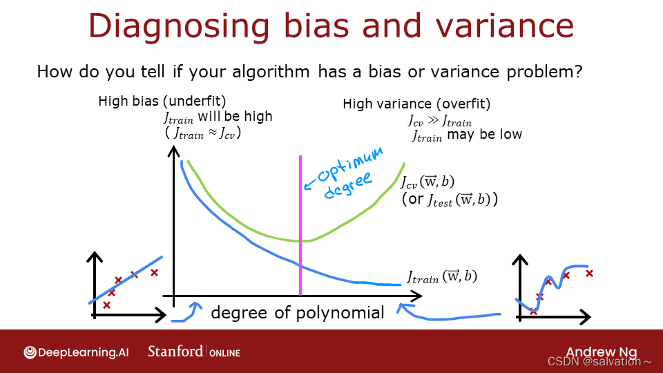
Above, it was clear the degree of the polynomial model was too high. How can you choose a good value? It turns out, as shown in the diagram, the training and cross-validation performance can provide guidance. By trying a range of degree values, the training and cross-validation performance can be evaluated. As the degree becomes too large, the cross-validation performance will start to degrade relative to the training performance. Let’s try this on our example.
由此可见,多项式模型的程度过高。如何选择性价比高的产品?事实证明,如图所示,训练和交叉验证性能可以提供指导。通过尝试一定范围的度值,可以评估训练和交叉验证的性能。当交叉验证的程度过大时,交叉验证的性能就会相对于训练性能开始下降。让我们在我们的例子中试试。
3.1 Plot Train, Cross-Validation, Test
You can see below the datapoints that will be part of training (in red) are intermixed with those that the model is not trained on (test and cv).
您可以在下面看到,将成为训练一部分的数据点(红色)与模型未训练的数据点(test和cv)混合在一起
fig, ax = plt.subplots(1,1,figsize=(4,4))
ax.plot(x_ideal, y_ideal, "--", color = "orangered", label="y_ideal", lw=1)
ax.set_title("Training, CV, Test",fontsize = 14)
ax.set_xlabel("x")
ax.set_ylabel("y")

ax.scatter(X_train, y_train, color = "red",           label="train")
ax.scatter(X_cv, y_cv,       color = dlc["dlorange"], label="cv")
ax.scatter(X_test, y_test,   color = dlc["dlblue"],   label="test")
ax.legend(loc='upper left')
plt.show()

3.2 Finding the optimal degree(寻找最优的度(度指次幂,如:
x
2
,
x
3
.
.
.
x^2,x^3 ...
x2,x3...))
In previous labs, you found that you could create a model capable of fitting complex curves by utilizing a polynomial (See Course1, Week2 Feature Engineering and Polynomial Regression Lab). Further, you demonstrated that by increasing the degree of the polynomial, you could create overfitting. (See Course 1, Week3, Over-Fitting Lab). Let’s use that knowledge here to test our ability to tell the difference between over-fitting and under-fitting.
在之前的实验室中,您找到了一种方法,可以通过使用多项式(参见课程1,第2周功能工程和多项式回归实验室)来创建能够拟合复杂曲线的模型。此外,您还演示了通过增加多项式的度,可以创建过度拟合。(参见课程1,第3周,过度拟合实验室)。让我们利用这些知识在这里来测试我们能够区分过拟合和欠拟合的能力。
Let’s train the model repeatedly, increasing the degree of the polynomial each iteration. Here, we’re going to use the scikit-learn linear regression model for speed and simplicity.
让我们重复地训练模型,每次迭代增加多项式的度。在这里,我们将使用scikit-learn线性回归模型,以速度和简单性。
max_degree = 9
err_train = np.zeros(max_degree)
err_cv = np.zeros(max_degree)
x = np.linspace(0,int(X.max()),100)
y_pred = np.zeros((100,max_degree))  #columns are lines to plot

for degree in range(max_degree):
    lmodel = lin_model(degree+1)
    lmodel.fit(X_train, y_train)
    yhat = lmodel.predict(X_train)
    err_train[degree] = lmodel.mse(y_train, yhat)
    yhat = lmodel.predict(X_cv)
    err_cv[degree] = lmodel.mse(y_cv, yhat)
    y_pred[:,degree] = lmodel.predict(x)

optimal_degree = np.argmin(err_cv)+1
Let’s plot the result:
plt.close("all")
plt_optimal_degree(X_train, y_train, X_cv, y_cv, x, y_pred, x_ideal, y_ideal,
                   err_train, err_cv, optimal_degree, max_degree)

The plot above demonstrates that separating data into two groups, data the model is trained on and data the model has not been trained on, can be used to determine if the model is underfitting or overfitting. In our example, we created a variety of models varying from underfitting to overfitting by increasing the degree of the polynomial used.
上图表明,将数据分为两组,即模型训练过的数据和模型未训练过的数据,可以用来确定模型是欠拟合还是过拟合。在我们的示例中,我们通过增加所使用的多项式的程度,创建了从欠拟合到过拟合的各种模型。
- On the left plot, the solid lines represent the predictions from these models. A polynomial model with degree 1 produces a straight line that intersects very few data points, while the maximum degree hews very closely to every data point.(左图中,实线表示这些模型的预测。具有1度的多项式模型产生一条与很少数据点相交的直线,而最大程度的模型非常接近每个数据点)
- on the right:
- the error on the trained data (blue) decreases as the model complexity increases as expected(随着模型复杂性的增加,训练数据的误差会降低,这是预期的)
- the error of the cross-validation data decreases initially as the model starts to conform to the data, but then increases as the model starts to over-fit on the training data (fails to generalize).(交叉验证数据的误差最初随着模型开始与数据相符而减小,然后随着模型开始与训练数据过拟合而增大(无法泛化)。)
It’s worth noting that the curves in these examples as not as smooth as one might draw for a lecture. It’s clear the specific data points assigned to each group can change your results significantly. The general trend is what is important.
值得注意的是,这些例子中的曲线并不像讲课时画的那么光滑。很明显,分配给每一组的特定数据点可以显著改变你的结果。大趋势才是最重要的。
3.3 Tuning Regularization.(调参正则化)
In previous labs, you have utilized regularization to reduce overfitting. Similar to degree, one can use the same methodology to tune the regularization parameter lambda (
λ
\lambda
λ).
在之前的实验中,您已经利用了正则化来减少过拟合。类似于度,您可以使用相同的方法来调整正则化参数lambda()。
Let’s demonstrate this by starting with a high degree polynomial and varying the regularization parameter.
首先,让我们通过从一个高阶多项式开始,并改变正则化参数来演示这一点。
```python
lambda_range = np.array([0.0, 1e-6, 1e-5, 1e-4,1e-3,1e-2, 1e-1,1,10,100])
num_steps = len(lambda_range)
degree = 10
err_train = np.zeros(num_steps)
err_cv = np.zeros(num_steps)
x = np.linspace(0,int(X.max()),100)
y_pred = np.zeros((100,num_steps))  #columns are lines to plot

for i in range(num_steps):
    lambda_= lambda_range[i]
    lmodel = lin_model(degree, regularization=True, lambda_=lambda_)
    lmodel.fit(X_train, y_train)
    yhat = lmodel.predict(X_train)
    err_train[i] = lmodel.mse(y_train, yhat)
    yhat = lmodel.predict(X_cv)
    err_cv[i] = lmodel.mse(y_cv, yhat)
    y_pred[:,i] = lmodel.predict(x)

optimal_reg_idx = np.argmin(err_cv)
plt.close("all")
plt_tune_regularization(X_train, y_train, X_cv, y_cv, x, y_pred, err_train, err_cv, optimal_reg_idx, lambda_range)

Above, the plots show that as regularization increases, the model moves from a high variance (overfitting) model to a high bias (underfitting) model. The vertical line in the right plot shows the optimal value of lambda. In this example, the polynomial degree was set to 10.
上面的图表显示,随着正则化的增加,模型从具有高方差(过拟合)的模型移动到具有高偏差(欠拟合)的模型。 右图中的垂直线显示了 lambda 的最优值。 在这个例子中,多项式度被设置为 10。
3.4 Getting more data: Increasing Training Set Size (m)(增加训练集大小:m)
When a model is overfitting (high variance), collecting additional data can improve performance. Let’s try that here.
当一个模型是过拟合(高方差)时,收集额外的数据可以提高性能。让我们在这里试试。
X_train, y_train, X_cv, y_cv, x, y_pred, err_train, err_cv, m_range,degree = tune_m()
plt_tune_m(X_train, y_train, X_cv, y_cv, x, y_pred, err_train, err_cv, m_range, degree)

The above plots show that when a model has high variance and is overfitting, adding more examples improves performance. Note the curves on the left plot. The final curve with the highest value of
m
m
m is a smooth curve that is in the center of the data. On the right, as the number of examples increases, the performance of the training set and cross-validation set converge to similar values. Note that the curves are not as smooth as one might see in a lecture. That is to be expected. The trend remains clear: more data improves generalization.
上面的图表明,当一个模型具有高方差和过拟合时,增加更多的样本可以提高性能。注意左图上的曲线。
m
m
m值最高的最后一条曲线是位于数据中心的平滑曲线。在右边,随着样本数量的增加,训练集和交叉验证集的性能收敛到相似的值。注意,这些曲线并不像你在课堂上看到的那样平滑。这是意料之中的。趋势仍然很明显:更多的数据可以提高归纳能力。
Note that adding more examples when the model has high bias (underfitting) does not improve performance.
注意,当模型具有高偏差(欠拟合)时,添加更多的例子并不能提高性能。
4 - Evaluating a Learning Algorithm (Neural Network)(评估学习算法(神经网络))
Above, you tuned aspects of a polynomial regression model. Here, you will work with a neural network model. Let’s start by creating a classification data set.
在上面的内容中,你调整了多项式回归模型的各个方面。在这里,你将使用一个神经网络模型。让我们从创建一个分类数据集开始。
4.1 Data Set
Run the cell below to generate a data set and split it into training, cross-validation (CV) and test sets. In this example, we’re increasing the percentage of cross-validation data points for emphasis.
运行下面的单元格,生成一个数据集并将其分为训练、交叉验证(CV)和测试集。在这个例子中,我们增加交叉验证数据点的百分比,以强调这一点。
# Generate and split data set
X, y, centers, classes, std = gen_blobs()

# split the data. Large CV population for demonstration
X_train, X_, y_train, y_ = train_test_split(X,y,test_size=0.50, random_state=1)
X_cv, X_test, y_cv, y_test = train_test_split(X_,y_,test_size=0.20, random_state=1)
print("X_train.shape:", X_train.shape, "X_cv.shape:", X_cv.shape, "X_test.shape:", X_test.shape)
X_train.shape: (400, 2) X_cv.shape: (320, 2) X_test.shape: (80, 2)
plt_train_eq_dist(X_train, y_train,classes, X_cv, y_cv, centers, std)

Above, you can see the data on the left. There are six clusters identified by color. Both training points (dots) and cross-validataion points (triangles) are shown. The interesting points are those that fall in ambiguous locations where either cluster might consider them members. What would you expect a neural network model to do? What would be an example of overfitting? underfitting?
在上面,您可以看到左侧的数据。按颜色分为六组。同时显示训练点(点)和交叉验证点(三角形)。有趣的是那些落在模糊位置的点,任何一个集群都可能认为它们是成员。你期望神经网络模型能做什么?例子是过拟合?欠拟合?
On the right is an example of an ‘ideal’ model, or a model one might create knowing the source of the data. The lines represent ‘equal distance’ boundaries where the distance between center points is equal. It’s worth noting that this model would “misclassify” roughly 8% of the total data set.
右边是一个“理想”模型的例子,或者是一个知道数据来源后可能创建的模型。这些线表示中心点之间的距离相等的“等距”边界。值得注意的是,这个模型会“错误分类”大约8%的总数据集。
4.2 Evaluating categorical model by calculating classification error(通过计算分类误差来评价分类模型)
The evaluation function for categorical models used here is simply the fraction of incorrect predictions:
这里使用的分类模型的评价函数只是不正确预测的比例
J
c
v
=
1
m
∑
i
=
0
m
−
1
{
1
,
if
y
^
(
i
)
≠
y
(
i
)
0
,
otherwise
J_{cv} =\frac{1}{m}\sum_{i=0}^{m-1} \begin{cases} 1, & \text{if $\hat{y}^{(i)} \neq y^{(i)}$}\\ 0, & \text{otherwise} \end{cases}
Jcv=m1i=0∑m−1{1,0,if y^(i)=y(i)otherwise
Exercise 2
Below, complete the routine to calculate classification error. Note, in this lab, target values are the index of the category and are not one-hot encoded.
在下面,完成计算分类误差的例程。注意,在本实验中,目标值是类别的索引,而不是独热编码。
# UNQ_C2
# GRADED CELL: eval_cat_err
def eval_cat_err(y, yhat):
    """
    Calculate the categorization error
    Args:
      y    : (ndarray  Shape (m,) or (m,1))  target value of each example
      yhat : (ndarray  Shape (m,) or (m,1))  predicted value of each example
    Returns:|
      cerr: (scalar)
    """
    m = len(y)
    incorrect = 0
    for i in range(m):
    ### START CODE HERE ###
      if yhat[i] != y[i]:
         incorrect +=1
      else:
         incorrect +=0
    ### END CODE HERE ###
    cerr = incorrect / m
    return(cerr)
y_hat = np.array([1, 2, 0])
y_tmp = np.array([1, 2, 3])
print(f"categorization error {np.squeeze(eval_cat_err(y_hat, y_tmp)):0.3f}, expected:0.333" )
y_hat = np.array([[1], [2], [0], [3]])
y_tmp = np.array([[1], [2], [1], [3]])
print(f"categorization error {np.squeeze(eval_cat_err(y_hat, y_tmp)):0.3f}, expected:0.250" )

# BEGIN UNIT TEST
test_eval_cat_err(eval_cat_err)
# END UNIT TEST
# BEGIN UNIT TEST
test_eval_cat_err(eval_cat_err)
# END UNIT TEST
categorization error 0.333, expected:0.333
categorization error 0.250, expected:0.250
[92m All tests passed.
[92m All tests passed.
def eval_cat_err(y, yhat):
    """
    Calculate the categorization error
    Args:
      y    : (ndarray  Shape (m,) or (m,1))  target value of each example
      yhat : (ndarray  Shape (m,) or (m,1))  predicted value of each example
    Returns:|
      cerr: (scalar)
    """
    m = len(y)
    incorrect = 0
    for i in range(m):
        if yhat[i] != y[i]:    # @REPLACE
            incorrect += 1     # @REPLACE
    cerr = incorrect/m         # @REPLACE
    return(cerr)
5 - Model Complexity
Below, you will build two models. A complex model and a simple model. You will evaluate the models to determine if they are likely to overfit or underfit.
下面,你将构建两个模型。一个复杂模型和一个简单模型。你将评估模型,以确定它们是否可能过度拟合或欠拟合。
5.1 Complex model
Exercise 3
Below, compose a three-layer model:
在下面,组成一个三层的模型:
- Dense layer with 120 units, relu activation
- Dense layer with 40 units, relu activation
- Dense layer with 6 units and a linear activation (not softmax)
Compile using - loss with
SparseCategoricalCrossentropy, remember to usefrom_logits=True - Adam optimizer with learning rate of 0.01.
# UNQ_C3
# GRADED CELL: model
import logging
logging.getLogger("tensorflow").setLevel(logging.ERROR)

tf.random.set_seed(1234)
model = Sequential(
    [
        ### START CODE HERE ###
        # tf.keras.Input(shape=(400,2)),
        Dense(120,activation='relu',input_shape=(X_train.shape[1],),name = 'L1'),
        Dense(40,activation='relu', name = 'L2'),
        Dense(classes,activation='linear',name = 'L3')
        ### END CODE HERE ###

    ], name="Complex"
)
model.compile(
    ### START CODE HERE ###
    loss=tf.keras.losses.SparseCategoricalCrossentropy(from_logits=True),
    optimizer=tf.keras.optimizers.Adam(learning_rate=0.01),
    ### END CODE HERE ###
)
# BEGIN UNIT TEST
model.fit(
    X_train, y_train,
    epochs=1000
)
# END UNIT TEST
Epoch 1/1000
13/13 [==============================] - 1s 997us/step - loss: 1.1106
...
Epoch 999/1000
13/13 [==============================] - 0s 914us/step - loss: 0.0334
Epoch 1000/1000
13/13 [==============================] - 0s 914us/step - loss: 0.0326


<keras.callbacks.History at 0x22b1f388280>
# BEGIN UNIT TEST
model.summary()

model_test(model, classes, X_train.shape[1])
# END UNIT TEST
Model: "Complex"
_________________________________________________________________
Layer (type)                 Output Shape              Param #
=================================================================
L1 (Dense)                   (None, 120)               360
_________________________________________________________________
L2 (Dense)                   (None, 40)                4840
_________________________________________________________________
L3 (Dense)                   (None, 6)                 246
=================================================================
Total params: 5,446
Trainable params: 5,446
Non-trainable params: 0
_________________________________________________________________
[92mAll tests passed!
Summary should match this (layer instance names may increment )
Model: "Complex"
_________________________________________________________________
Layer (type)                 Output Shape              Param #
=================================================================
L1 (Dense)                   (None, 120)               360
_________________________________________________________________
L2 (Dense)                   (None, 40)                4840
_________________________________________________________________
L3 (Dense)                   (None, 6)                 246
=================================================================
Total params: 5,446
Trainable params: 5,446
Non-trainable params: 0
_________________________________________________________________
tf.random.set_seed(1234)
model = Sequential(
    [
        Dense(120, activation = 'relu', name = "L1"),
        Dense(40, activation = 'relu', name = "L2"),
        Dense(classes, activation = 'linear', name = "L3")
    ], name="Complex"
)
model.compile(
    loss=tf.keras.losses.SparseCategoricalCrossentropy(from_logits=True),
    optimizer=tf.keras.optimizers.Adam(0.01),
)

model.fit(
    X_train,y_train,
    epochs=1000
)
#make a model for plotting routines to call
model_predict = lambda Xl: np.argmax(tf.nn.softmax(model.predict(Xl)).numpy(),axis=1)
plt_nn(model_predict,X_train,y_train, classes, X_cv, y_cv, suptitle="Complex Model")

This model has worked very hard to capture outliers of each category. As a result, it has miscategorized some of the cross-validation data. Let’s calculate the classification error.
这个模型非常努力地捕捉每一类别的异常值。因此,它错误地分类了一些交叉验证数据。让我们计算一下分类误差。
training_cerr_complex = eval_cat_err(y_train, model_predict(X_train))
cv_cerr_complex = eval_cat_err(y_cv, model_predict(X_cv))
print(f"categorization error, training, complex model: {training_cerr_complex:0.3f}")
print(f"categorization error, cv,       complex model: {cv_cerr_complex:0.3f}")
categorization error, training, complex model: 0.015
categorization error, cv,       complex model: 0.122
5.1 Simple model(简单模型)
Now, let’s try a simple model
现在,让我们尝试一个简单的模型
Exercise 4
Below, compose a two-layer model:
- Dense layer with 6 units, relu activation
- Dense layer with 6 units and a linear activation.
Compile using - loss with
SparseCategoricalCrossentropy, remember to usefrom_logits=True - Adam optimizer with learning rate of 0.01.
# UNQ_C4
# GRADED CELL: model_s

tf.random.set_seed(1234)
model_s = Sequential(
    [
        ### START CODE HERE ###
        Dense(6, activation='relu', input_shape=(X_train.shape[1],)),
        Dense(6,activation='linear'),
        ### END CODE HERE ###
    ], name = "Simple"
)
model_s.compile(
    ### START CODE HERE ###
    loss=SparseCategoricalCrossentropy(from_logits=True),
    optimizer=tf.keras.optimizers.Adam(learning_rate=0.01)
    ### START CODE HERE ###
)
import logging
logging.getLogger("tensorflow").setLevel(logging.ERROR)

# BEGIN UNIT TEST
model_s.fit(
    X_train,y_train,
    epochs=1000
)
# END UNIT TEST
Epoch 1/1000
13/13 [==============================] - 0s 831us/step - loss: 1.7306
...
Epoch 999/1000
13/13 [==============================] - 0s 664us/step - loss: 0.1711
Epoch 1000/1000
13/13 [==============================] - 0s 748us/step - loss: 0.1628


<keras.callbacks.History at 0x22b8f2be940>
# BEGIN UNIT TEST
model_s.summary()

model_s_test(model_s, classes, X_train.shape[1])
# END UNIT TEST
Model: "Simple"
_________________________________________________________________
Layer (type)                 Output Shape              Param #
=================================================================
dense (Dense)                (None, 6)                 18
_________________________________________________________________
dense_1 (Dense)              (None, 6)                 42
=================================================================
Total params: 60
Trainable params: 60
Non-trainable params: 0
_________________________________________________________________
[92mAll tests passed!
Summary should match this (layer instance names may increment )
Model: "Simple"
_________________________________________________________________
Layer (type)                 Output Shape              Param #
=================================================================
L1 (Dense)                   (None, 6)                 18
_________________________________________________________________
L2 (Dense)                   (None, 6)                 42
=================================================================
Total params: 60
Trainable params: 60
Non-trainable params: 0
_________________________________________________________________
tf.random.set_seed(1234)
model_s = Sequential(
    [
        Dense(6, activation = 'relu', name="L1"),            # @REPLACE
        Dense(classes, activation = 'linear', name="L2")     # @REPLACE
    ], name = "Simple"
)
model_s.compile(
    loss=tf.keras.losses.SparseCategoricalCrossentropy(from_logits=True),     # @REPLACE
    optimizer=tf.keras.optimizers.Adam(0.01),     # @REPLACE
)

model_s.fit(
    X_train,y_train,
    epochs=1000
)
#make a model for plotting routines to call
model_predict_s = lambda Xl: np.argmax(tf.nn.softmax(model_s.predict(Xl)).numpy(),axis=1)
plt_nn(model_predict_s,X_train,y_train, classes, X_cv, y_cv, suptitle="Simple Model")

This simple models does pretty well. Let’s calculate the classification error.
这个简单的模型做得很好。让我们计算一下分类误差
training_cerr_simple = eval_cat_err(y_train, model_predict_s(X_train))
cv_cerr_simple = eval_cat_err(y_cv, model_predict_s(X_cv))
print(f"categorization error, training, simple model, {training_cerr_simple:0.3f}, complex model: {training_cerr_complex:0.3f}" )
print(f"categorization error, cv,       simple model, {cv_cerr_simple:0.3f}, complex model: {cv_cerr_complex:0.3f}" )
categorization error, training, simple model, 0.062, complex model: 0.015
categorization error, cv, simple model, 0.087, complex model: 0.122
Our simple model has a little higher classification error on training data but does better on cross-validation data than the more complex model.
我们的简单模型在训练数据上有更高的分类误差,但在交叉验证数据上比更复杂的模型做得更好
6 - Regularization(正则化)
As in the case of polynomial regression, one can apply regularization to moderate the impact of a more complex model. Let’s try this below.
就像多项式回归的情况一样,我们可以对更复杂的模型进行正则化,以中和其影响。让我们试着这样做。
Exercise 5
Reconstruct your complex model, but this time include regularization.
重建您的复杂模型,但这一次包括正则化。
Below, compose a three-layer model:
- Dense layer with 120 units, relu activation,
kernel_regularizer=tf.keras.regularizers.l2(0.1) - Dense layer with 40 units, relu activation,
kernel_regularizer=tf.keras.regularizers.l2(0.1) - Dense layer with 6 units and a linear activation.
Compile using - loss with
SparseCategoricalCrossentropy, remember to usefrom_logits=True - Adam optimizer with learning rate of 0.01.
# UNQ_C5
# GRADED CELL: model_r

tf.random.set_seed(1234)
model_r = Sequential(
    [
        ### START CODE HERE ###
        Dense(120,activation='relu',kernel_regularizer=tf.keras.regularizers.l2(0.1)),
        Dense(40,activation='relu',kernel_regularizer=tf.keras.regularizers.l2(0.1)),
        Dense(6,activation='linear')
        ### START CODE HERE ###
    ], name= None
)
model_r.compile(
    ### START CODE HERE ###
    loss=SparseCategoricalCrossentropy(from_logits= True),
    optimizer=tf.keras.optimizers.Adam(learning_rate=0.01),
    ### START CODE HERE ###
)
# BEGIN UNIT TEST
model_r.fit(
    X_train, y_train,
    epochs=1000
)
# END UNIT TEST
Epoch 1/1000
13/13 [==============================] - 0s 3ms/step - loss: 4.4464
...
Epoch 999/1000
13/13 [==============================] - 0s 997us/step - loss: 0.3505
Epoch 1000/1000
13/13 [==============================] - 0s 997us/step - loss: 0.3514


<keras.callbacks.History at 0x27b901affa0>
# BEGIN UNIT TEST
model_r.summary()

model_r_test(model_r, classes, X_train.shape[1])
# END UNIT TEST
Model: "sequential"
_________________________________________________________________
Layer (type)                 Output Shape              Param #
=================================================================
dense_2 (Dense)              (None, 120)               360
_________________________________________________________________
dense_3 (Dense)              (None, 40)                4840
_________________________________________________________________
dense_4 (Dense)              (None, 6)                 246
=================================================================
Total params: 5,446
Trainable params: 5,446
Non-trainable params: 0
_________________________________________________________________
ddd
[92mAll tests passed!
Summary should match this (layer instance names may increment )
Model: "ComplexRegularized"
_________________________________________________________________
Layer (type)                 Output Shape              Param #
=================================================================
L1 (Dense)                   (None, 120)               360
_________________________________________________________________
L2 (Dense)                   (None, 40)                4840
_________________________________________________________________
L3 (Dense)                   (None, 6)                 246
=================================================================
Total params: 5,446
Trainable params: 5,446
Non-trainable params: 0
_________________________________________________________________
tf.random.set_seed(1234)
model_r = Sequential(
    [
        Dense(120, activation = 'relu', kernel_regularizer=tf.keras.regularizers.l2(0.1), name="L1"),
        Dense(40, activation = 'relu', kernel_regularizer=tf.keras.regularizers.l2(0.1), name="L2"),
        Dense(classes, activation = 'linear', name="L3")
    ], name="ComplexRegularized"
)
model_r.compile(
    loss=tf.keras.losses.SparseCategoricalCrossentropy(from_logits=True),
    optimizer=tf.keras.optimizers.Adam(0.01),
)

model_r.fit(
    X_train,y_train,
    epochs=1000
)
#make a model for plotting routines to call
model_predict_r = lambda Xl: np.argmax(tf.nn.softmax(model_r.predict(Xl)).numpy(),axis=1)

plt_nn(model_predict_r, X_train,y_train, classes, X_cv, y_cv, suptitle="Regularized")

The results look very similar to the ‘ideal’ model. Let’s check classification error.
结果看起来和“理想”模型非常相似。让我们检查一下分类误差。
training_cerr_reg = eval_cat_err(y_train, model_predict_r(X_train))
cv_cerr_reg = eval_cat_err(y_cv, model_predict_r(X_cv))
test_cerr_reg = eval_cat_err(y_test, model_predict_r(X_test))
print(f"categorization error, training, regularized: {training_cerr_reg:0.3f}, simple model, {training_cerr_simple:0.3f}, complex model: {training_cerr_complex:0.3f}" )
print(f"categorization error, cv,       regularized: {cv_cerr_reg:0.3f}, simple model, {cv_cerr_simple:0.3f}, complex model: {cv_cerr_complex:0.3f}" )
categorization error, training, regularized: 0.072, simple model, 0.062, complex model: 0.015
categorization error, cv, regularized: 0.066, simple model, 0.087, complex model: 0.122
The simple model is a bit better in the training set than the regularized model but it worse in the cross validation set.
这个简单的模型在训练集中比正则化的模型略好,但在交叉验证集中更差。
7 - Iterate to find optimal regularization value(迭代找到最优正则化值)
As you did in linear regression, you can try many regularization values. This code takes several minutes to run. If you have time, you can run it and check the results. If not, you have completed the graded parts of the assignment!
就像你在线性回归中做的那样,你可以尝试很多正则化值。这段代码运行需要几分钟。如果你有时间,你可以运行它并检查结果。如果你没有时间,你已经完成了这个作业的评分部分!
tf.random.set_seed(1234)
lambdas = [0.0, 0.001, 0.01, 0.05, 0.1, 0.2, 0.3]
models=[None] * len(lambdas)
for i in range(len(lambdas)):
    lambda_ = lambdas[i]
    models[i] =  Sequential(
        [
            Dense(120, activation = 'relu', kernel_regularizer=tf.keras.regularizers.l2(lambda_)),
            Dense(40, activation = 'relu', kernel_regularizer=tf.keras.regularizers.l2(lambda_)),
            Dense(classes, activation = 'linear')
        ]
    )
    models[i].compile(
        loss=tf.keras.losses.SparseCategoricalCrossentropy(from_logits=True),
        optimizer=tf.keras.optimizers.Adam(0.01),
    )

    models[i].fit(
        X_train,y_train,
        epochs=1000
    )
    print(f"Finished lambda = {lambda_}")
Epoch 1/1000
13/13 [==============================] - 0s 1ms/step - loss: 1.1106
Epoch 2/1000
13/13 [==============================] - 0s 1ms/step - loss: 0.4281
...
Epoch 999/1000
13/13 [==============================] - 0s 1ms/step - loss: 0.4226
Epoch 1000/1000
13/13 [==============================] - 0s 997us/step - loss: 0.4582
Finished lambda = 0.3
plot_iterate(lambdas, models, X_train, y_train, X_cv, y_cv)

As regularization is increased, the performance of the model on the training and cross-validation data sets converge. For this data set and model, lambda > 0.01 seems to be a reasonable choice.
随着正则化的增加,模型在训练和交叉验证数据集上的性能收敛。对于这个数据集和模型,lambda > 0.01似乎是一个合理的选择。
7.1 Test
Let’s try our optimized models on the test set and compare them to ‘ideal’ performance.
让我们在测试集上尝试我们优化的模型,并将它们与“理想”性能进行比较
plt_compare(X_test,y_test, classes, model_predict_s, model_predict_r, centers)

Our test set is small and seems to have a number of outliers so classification error is high. However, the performance of our optimized models is comparable to ideal performance.
我们的测试集很小,似乎有很多离群值,因此分类误差很高。然而,我们优化的模型的性能与理想性能相当。
Congratulations(恭喜)!
You have become familiar with important tools to apply when evaluating your machine learning models. Namely:
您已经熟悉了在评估机器学习模型时应用的重要工具。即:
- splitting data into trained and untrained sets allows you to differentiate between underfitting and overfitting(将数据分为已训练和未训练的集合允许您区分欠拟合和过拟合)
- creating three data sets, Training, Cross-Validation and Test allows you to(创建三个数据集,训练,交叉验证和测试允许您)
- train your parameters W , B W,B W,B with the training set(使用训练集训练参数 W , B W,B W,B)
- tune model parameters such as complexity, regularization and number of examples with the cross-validation set(使用交叉验证集调整模型参数,如复杂性,正则化和示例数量)
- evaluate your ‘real world’ performance using the test set.(使用测试集评估“真实世界”性能)
- comparing training vs cross-validation performance provides insight into a model’s propensity towards overfitting (high variance) or underfitting (high bias)(比较训练和交叉验证性能提供了有关模型过度拟合(高方差)或欠拟合(高偏差)的倾向的见解)
下面我们使用Pytorch来实现带有正则化的回归模型。
目标:
- 了解过拟合(高方差)和欠拟合(高偏差),以及该采取的措施
- 将数据集划分为训练集和测试集,验证集
- 实现带有正则化的模型,并判断其性能
| 问题名称 | 解决方法 |
|---|---|
| 高方差(过拟合) | 使用更多的训练集,减少模型复杂度,增大正则化系数 |
| 高偏差(欠拟合) | 增加模型复杂度,添加特征,减小正则化系数 |
接下里,我们导入我们需要使用的包
import torch
import torchvision
from torch.utils.data import DataLoader,TensorDataset,random_split
from torch.utils.tensorboard import SummaryWriter
from torch import nn
import numpy as np
from sklearn.datasets import make_blobs
import random
采用gpu训练可以更快。
# 定义训练设备
device = torch.device("cuda" if torch.cuda.is_available() else "cpu")
创建数据集
def gen_blobs():
    classes = 6
    m = 800
    std = 0.4
    centers = np.array([[-1, 0], [1, 0], [0, 1], [0, -1],  [-2,1],[-2,-1]])
    X, y = make_blobs(n_samples=m, centers=centers, cluster_std=std, random_state=2, n_features=2)
    return (X, y, centers, classes, std)
#创建数据集
X, y, centers, classes, std = gen_blobs()

X = torch.tensor(X,dtype=torch.float32)
y = torch.tensor(y,dtype=torch.long)

#获取数据的长度
dataset = TensorDataset(X,y)
len_dataset = len(dataset)
len_train_dataset = int(0.6*len_dataset)
len_test_dataset = len_dataset - len_train_dataset
#将数据集分为训练集和测试集
train_dataset, test_dataset = random_split(dataset,[len_train_dataset,len_test_dataset])

dataloader_train = DataLoader(train_dataset,batch_size=1,shuffle=True)
dataloader_test = DataLoader(test_dataset,batch_size=1,shuffle=True)

# 查看train_dataset和test_dataset的形状
print(train_dataset.dataset.tensors[0].shape)
torch.Size([800, 2])
通过运行结果我们可以知道,训练集的形状为(800, 2),测试集的形状为(200, 2)。以此来定义第一层线性层输入的值
#---------------------------------------------------#
#   设置种子
#---------------------------------------------------#
# 设置随机种子,使每次运行的结果相同
def seed_everything(seed=11):
    # 设置随机数种子
    random.seed(seed)
    # 设置numpy的随机数种子
    np.random.seed(seed)
    # 设置torch的随机数种子
    torch.manual_seed(seed)
    # 设置torch.cuda的随机数种子
    torch.cuda.manual_seed(seed)
    # 设置torch.cuda中所有设备上的随机数种子
    torch.cuda.manual_seed_all(seed)
    # 设置cudnn的随机数种子
    torch.backends.cudnn.deterministic = True
    torch.backends.cudnn.benchmark = False
seed_everything()
#构建网络模型
class NetComplex(nn.Module):
    def __init__(self):
        super(NetComplex,self).__init__()
        self.model = nn.Sequential(
            nn.Linear(2, 120),
            nn.ReLU(),
            nn.Linear(120, 40),
            nn.ReLU(),
            nn.Linear(40, classes)
        )


    def forward(self,x):
        x = self.model(x)
        return x
有正则化项的代价函数如下:
J
(
w
,
b
)
=
1
2
m
∑
i
=
0
m
−
1
(
f
w
,
b
(
x
(
i
)
)
−
y
(
i
)
)
2
+
λ
2
m
∑
j
=
0
n
−
1
w
j
2
(1)
J(\mathbf{w},b) = \frac{1}{2m} \sum\limits_{i = 0}^{m-1} (f_{\mathbf{w},b}(\mathbf{x}^{(i)}) - y^{(i)})^2 + \frac{\lambda}{2m} \sum_{j=0}^{n-1} w_j^2 \tag{1}
J(w,b)=2m1i=0∑m−1(fw,b(x(i))−y(i))2+2mλj=0∑n−1wj2(1)
在pytorch中l2正则化,可以通过对优化器添加weight_decay(就相当于
λ
\lambda
λ)参数来实现,在下面我们会使用两个神经网络模型(一个有正则化,一个没有正则化)来对比
# 构建两个模型一个有正则化一个没有正则化
model_re = NetComplex()
model_no_re = NetComplex()

#损失函数
loss = nn.CrossEntropyLoss()

#优化器,weight_decay相当于正则化系数
learning_rate = 1e-2
optimizer_re = torch.optim.Adam(model_re.parameters(),lr=0.01,weight_decay=0.01)
optimizer_no_re = torch.optim.Adam(model_no_re.parameters(),lr=0.01)

#训练次数和测试次数
total_train_step = 0
total_test_step = 0

#训练轮数
epoch = 50

#添加tensorboard
writer = SummaryWriter("logs_re_nore")

for i in range(epoch):
    print("---------第{}轮训练开始---------".format(i+1))

    model_re.train()
    for data in dataloader_train:
        imgs,labels = data
        Output_re = model_re(imgs)
        ouput = model_no_re(imgs)
        loss_re = loss(Output_re,labels)
        loss_no_re = loss(ouput,labels)

        optimizer_re.zero_grad()
        optimizer_no_re.zero_grad()
        loss_re.backward()
        loss_no_re.backward()
        optimizer_re.step()
        optimizer_no_re.step()

        total_train_step += 1
        if total_train_step % 100 == 0:
            print("训练次数:{},loss_re:{}".format(total_train_step,loss_re.item()))
            print("训练次数:{},loss_no_re:{}".format(total_train_step,loss_no_re.item()))
            writer.add_scalar("train_loss_re",loss_re.item(),total_train_step)
            writer.add_scalar("train_loss_no_re",loss_no_re.item(),total_train_step)

    #测试步骤开始
    model_re.eval()
    total_test_loss_no_re = 0
    total_test_loss_re = 0
    accuracy_re = 0
    accuracy_no_re = 0
    total_accuracy_re = 0
    total_accuracy_no_re = 0
    with torch.no_grad():
        for data in dataloader_test:
            imgs,labels = data
            Output_re = model_re(imgs)
            Ouput = model_no_re(imgs)
            loss_re = loss(Output_re,labels)
            loss_no_re = loss(Ouput,labels)
            total_test_loss_no_re += loss_no_re.item()
            total_test_loss_re += loss_re.item()
            accuracy_re = (Output_re.argmax(dim=1) == labels).sum()
            accuracy_no_re = (Ouput.argmax(dim=1) == labels).sum()
            total_accuracy_re += accuracy_re
            total_accuracy_no_re += accuracy_no_re

    print("整体测试集上的Loss_no_re:{}".format(total_test_loss_no_re))
    print("整体本测试集上的Loss_re:{}".format(total_test_loss_re))
    print("整体测试集上的Accuracy_no_re:{}".format(total_accuracy_no_re / len(dataloader_test)))
    print("整体测试集上的Accuracy_re:{}".format(total_accuracy_re / len(dataloader_test)))
    writer.add_scalar("test_loss_re",total_test_loss_re,total_test_step)
    writer.add_scalar("test_loss_no_re",total_test_loss_no_re,total_test_step)
    writer.add_scalar("test_accuracy_re",total_accuracy_re / len(dataloader_test),total_test_step)
    writer.add_scalar("test_accuracy_no_re",total_accuracy_no_re / len(dataloader_test),total_test_step)
    total_test_step +=1


    if i == 6:
        torch.save(model_re.state_dict(), "model_re_dict{}.pth".format(i+1))
        print("模型已保存")


writer.close()
---------第1轮训练开始---------
训练次数:100,loss_re:2.7755062580108643
训练次数:100,loss_no_re:3.9803855419158936
训练次数:200,loss_re:0.011493775062263012
训练次数:200,loss_no_re:0.001423299196176231
训练次数:300,loss_re:0.6258141994476318
...
---------第50轮训练开始---------
训练次数:23600,loss_re:0.016745246946811676
训练次数:23600,loss_no_re:4.339123915997334e-05
...
训练次数:24000,loss_no_re:0.2639411389827728
整体测试集上的Loss_no_re:176.11682324294918
整体本测试集上的Loss_re:94.82983099698322
整体测试集上的Accuracy_no_re:0.875
整体测试集上的Accuracy_re:0.909375011920929

通过tensorboard可视化的结果我们可以清楚的看到,正则化带来的效果是显著的。


 被折叠的 条评论
为什么被折叠?
被折叠的 条评论
为什么被折叠?
 到【灌水乐园】发言


