iotdb分段分组聚合_iotdb 聚合统计

2401_83703951
于 2024-05-13 15:06:44 发布
阅读量173
点赞数 3
分类专栏：程序员文章标签： iotdb 数据库
本文链接：https://blog.csdn.net/2401_83703951/article/details/138803949
版权
程序员专栏收录该内容
451 篇文章 2 订阅
订阅专栏
±----------------------------±------------------------------±---------------------------------------+
Total line number = 5
It costs 0.006s
#按照自然月份的时间区间分组聚合查询
对应的 SQL 语句是：
select count(status) from root.ln.wf01.wt01 where time > 2017-11-01T01:00:00
group by([2017-11-01T00:00:00, 2019-11-07T23:00:00), 1mo, 2mo);
这条查询的含义是：
由于用户指定了滑动步长为2mo，GROUP BY 语句执行时将会每次把时间间隔往后移动 2 个自然月的步长，而不是默认的 1 个自然月。
也就意味着，我们想要取从 2017-11-01 到 2019-11-07 每 2 个自然月的第一个月的数据。

上面这个例子的第一个参数是显示窗口参数，决定了最终的显示范围是 [2017-11-01T00:00:00, 2019-11-07T23:00:00)。


起始时间为 2017-11-01T00:00:00，滑动步长将会以起始时间作为标准按月递增，取当月的 1 号作为时间间隔的起始时间。


上面这个例子的第二个参数是划分时间轴的时间间隔参数，将1mo当作划分间隔，显示窗口参数的起始时间当作分割原点，时间轴即被划分为连续的时间间隔：[2017-11-01T00:00:00, 2017-12-01T00:00:00), [2018-02-01T00:00:00, 2018-03-01T00:00:00), [2018-05-03T00:00:00, 2018-06-01T00:00:00) 等等。


上面这个例子的第三个参数是每次时间间隔的滑动步长。


然后系统将会用 WHERE 子句中的时间和值过滤条件以及 GROUP BY 语句中的第一个参数作为数据的联合过滤条件，获得满足所有过滤条件的数据（在这个例子里是在 [2017-11-01T00:00:00, 2019-11-07T23:00:00) 这个时间范围的数据），并把这些数据映射到之前分割好的时间轴中（这个例子里是从 2017-11-01T00:00:00 到 2019-11-07T23:00:00:00 的每两个自然月的第一个月）


每个时间间隔窗口内都有数据，SQL 执行后的结果集如下所示：


±----------------------------±------------------------------+  
 | Time|count(root.ln.wf01.wt01.status)|  
 ±----------------------------±------------------------------+  
 |2017-11-01T00:00:00.000+08:00| 259|  
 |2018-01-01T00:00:00.000+08:00| 250|  
 |2018-03-01T00:00:00.000+08:00| 259|  
 |2018-05-01T00:00:00.000+08:00| 251|  
 |2018-07-01T00:00:00.000+08:00| 242|  
 |2018-09-01T00:00:00.000+08:00| 225|  
 |2018-11-01T00:00:00.000+08:00| 216|  
 |2019-01-01T00:00:00.000+08:00| 207|  
 |2019-03-01T00:00:00.000+08:00| 216|  
 |2019-05-01T00:00:00.000+08:00| 207|  
 |2019-07-01T00:00:00.000+08:00| 199|  
 |2019-09-01T00:00:00.000+08:00| 181|  
 |2019-11-01T00:00:00.000+08:00| 60|  
 ±----------------------------±------------------------------+  
 对应的 SQL 语句是：


select count(status) from root.ln.wf01.wt01 group by([2017-10-31T00:00:00, 2019-11-07T23:00:00), 1mo, 2mo);  
 这条查询的含义是：


由于用户指定了滑动步长为2mo，GROUP BY 语句执行时将会每次把时间间隔往后移动 2 个自然月的步长，而不是默认的 1 个自然月。


也就意味着，我们想要取从 2017-10-31 到 2019-11-07 每 2 个自然月的第一个月的数据。


与上述示例不同的是起始时间为 2017-10-31T00:00:00，滑动步长将会以起始时间作为标准按月递增，取当月的 31 号（即最后一天）作为时间间隔的起始时间。若起始时间设置为 30 号，滑动步长会将时间间隔的起始时间设置为当月 30 号，若不存在则为最后一天。


上面这个例子的第一个参数是显示窗口参数，决定了最终的显示范围是 [2017-10-31T00:00:00, 2019-11-07T23:00:00)。


上面这个例子的第二个参数是划分时间轴的时间间隔参数，将1mo当作划分间隔，显示窗口参数的起始时间当作分割原点，时间轴即被划分为连续的时间间隔：[2017-10-31T00:00:00, 2017-11-31T00:00:00), [2018-02-31T00:00:00, 2018-03-31T00:00:00), [2018-05-31T00:00:00, 2018-06-31T00:00:00) 等等。


上面这个例子的第三个参数是每次时间间隔的滑动步长。


然后系统将会用 WHERE 子句中的时间和值过滤条件以及 GROUP BY 语句中的第一个参数作为数据的联合过滤条件，获得满足所有过滤条件的数据（在这个例子里是在 [2017-10-31T00:00:00, 2019-11-07T23:00:00) 这个时间范围的数据），并把这些数据映射到之前分割好的时间轴中（这个例子里是从 2017-10-31T00:00:00 到 2019-11-07T23:00:00:00 的每两个自然月的第一个月）


每个时间间隔窗口内都有数据，SQL 执行后的结果集如下所示：


±----------------------------±------------------------------+  
 | Time|count(root.ln.wf01.wt01.status)|  
 ±----------------------------±------------------------------+  
 |2017-10-31T00:00:00.000+08:00| 251|  
 |2017-12-31T00:00:00.000+08:00| 250|  
 |2018-02-28T00:00:00.000+08:00| 259|  
 |2018-04-30T00:00:00.000+08:00| 250|  
 |2018-06-30T00:00:00.000+08:00| 242|  
 |2018-08-31T00:00:00.000+08:00| 225|  
 |2018-10-31T00:00:00.000+08:00| 216|  
 |2018-12-31T00:00:00.000+08:00| 208|  
 |2019-02-28T00:00:00.000+08:00| 216|  
 |2019-04-30T00:00:00.000+08:00| 208|  
 |2019-06-30T00:00:00.000+08:00| 199|  
 |2019-08-31T00:00:00.000+08:00| 181|  
 |2019-10-31T00:00:00.000+08:00| 69|  
 ±----------------------------±------------------------------+  
 #左开右闭区间  
 每个区间的结果时间戳为区间右端点，对应的 SQL 语句是：


select count(status) from root.ln.wf01.wt01 group by ((2017-11-01T00:00:00, 2017-11-07T23:00:00],1d);  
 这条查询语句的时间区间是左开右闭的，结果中不会包含时间点 2017-11-01 的数据，但是会包含时间点 2017-11-07 的数据。


SQL 执行后的结果集如下所示：


±----------------------------±------------------------------+  
 | Time|count(root.ln.wf01.wt01.status)|  
 ±----------------------------±------------------------------+  
 |2017-11-02T00:00:00.000+08:00| 1440|  
 |2017-11-03T00:00:00.000+08:00| 1440|  
 |2017-11-04T00:00:00.000+08:00| 1440|  
 |2017-11-05T00:00:00.000+08:00| 1440|  
 |2017-11-06T00:00:00.000+08:00| 1440|  
 |2017-11-07T00:00:00.000+08:00| 1440|  
 |2017-11-07T23:00:00.000+08:00| 1380|  
 ±----------------------------±------------------------------+  
 Total line number = 7  
 It costs 0.004s  
 #与分组聚合混合使用  
 通过定义 LEVEL 来统计指定层级下的数据点个数。


例如：


统计降采样后的数据点个数


select count(status) from root.ln.wf01.wt01 group by ((2017-11-01T00:00:00, 2017-11-07T23:00:00],1d), level=1;  
 结果：


±----------------------------±------------------------+  
 | Time|COUNT(root.ln.*.*.status)|  
 ±----------------------------±------------------------+  
 |2017-11-02T00:00:00.000+08:00| 1440|  
 |2017-11-03T00:00:00.000+08:00| 1440|  
 |2017-11-04T00:00:00.000+08:00| 1440|  
 |2017-11-05T00:00:00.000+08:00| 1440|  
 |2017-11-06T00:00:00.000+08:00| 1440|  
 |2017-11-07T00:00:00.000+08:00| 1440|  
 |2017-11-07T23:00:00.000+08:00| 1380|  
 ±----------------------------±------------------------+  
 Total line number = 7  
 It costs 0.006s  
 加上滑动 Step 的降采样后的结果也可以汇总


select count(status) from root.ln.wf01.wt01 group by ([2017-11-01 00:00:00, 2017-11-07 23:00:00), 3h, 1d), level=1;


±----------------------------±------------------------+  
 | Time|COUNT(root.ln.*.*.status)|  
 ±----------------------------±------------------------+  
 |2017-11-01T00:00:00.000+08:00| 180|  
 |2017-11-02T00:00:00.000+08:00| 180|  
 |2017-11-03T00:00:00.000+08:00| 180|  
 |2017-11-04T00:00:00.000+08:00| 180|  
 |2017-11-05T00:00:00.000+08:00| 180|  
 |2017-11-06T00:00:00.000+08:00| 180|  
 |2017-11-07T00:00:00.000+08:00| 180|  
 ±----------------------------±------------------------+  
 Total line number = 7  
 It costs 0.004s  
 #路径层级分组聚合  
 在时间序列层级结构中，分层聚合查询用于对某一层级下同名的序列进行聚合查询。


使用 GROUP BY LEVEL = INT 来指定需要聚合的层级，并约定 ROOT 为第 0 层。若统计 “root.ln” 下所有序列则需指定 level 为 1。  
 分层聚合查询支持使用所有内置聚合函数。对于 sum，avg，min\_value， max\_value， extreme 五种聚合函数，需保证所有聚合的时间序列数据类型相同。其他聚合函数没有此限制。  
 示例1： 不同 database 下均存在名为 status 的序列， 如 “root.ln.wf01.wt01.status”, “root.ln.wf02.wt02.status”, 以及 “root.sgcc.wf03.wt01.status”, 如果需要统计不同 database 下 status 序列的数据点个数，使用以下查询：


select count(status) from root.\*\* group by level = 1  
 运行结果为：


±------------------------±--------------------------+  
 |count(root.ln.*.*.status)|count(root.sgcc.*.*.status)|  
 ±------------------------±--------------------------+  
 | 20160| 10080|  
 ±------------------------±--------------------------+  
 Total line number = 1  
 It costs 0.003s  
 示例2： 统计不同设备下 status 序列的数据点个数，可以规定 level = 3，


select count(status) from root.\*\* group by level = 3  
 运行结果为：


±--------------------------±--------------------------+  
 |count(root.*.*.wt01.status)|count(root.*.*.wt02.status)|  
 ±--------------------------±--------------------------+  
 | 20160| 10080|  
 ±--------------------------±--------------------------+  
 Total line number = 1  
 It costs 0.003s  
 注意，这时会将 database ln 和 sgcc 下名为 wt01 的设备视为同名设备聚合在一起。


示例3： 统计不同 database 下的不同设备中 status 序列的数据点个数，可以使用以下查询：


select count(status) from root.\*\* group by level = 1, 3  
 运行结果为：


±---------------------------±---------------------------±-----------------------------+  
 |count(root.ln.*.wt01.status)|count(root.ln.*.wt02.status)|count(root.sgcc.\*.wt01.status)|  
 ±---------------------------±---------------------------±-----------------------------+  
 | 10080| 10080| 10080|  
 ±---------------------------±---------------------------±-----------------------------+  
 Total line number = 1  
 It costs 0.003s  
 示例4： 查询所有序列下温度传感器 temperature 的最大值，可以使用下列查询语句：


select max\_value(temperature) from root.\*\* group by level = 0  
 运行结果：


±--------------------------------+  
 |max\_value(root.*.*.\*.temperature)|  
 ±--------------------------------+  
 | 26.0|  
 ±--------------------------------+  
 Total line number = 1  
 It costs 0.013s  
 示例5： 上面的查询都是针对某一个传感器，特别地，如果想要查询某一层级下所有传感器拥有的总数据点数，则需要显式规定测点为 \*


select count(\*) from root.ln.\*\* group by level = 2  
 运行结果：


±---------------------±---------------------+  
 |count(root.*.wf01.*.*)|count(root.*.wf02.*.*)|  
 ±---------------------±---------------------+  
 | 20160| 20160|  
 ±---------------------±---------------------+  
 Total line number = 1  
 It costs 0.013s  
 #标签分组聚合  
 IoTDB 支持通过 GROUP BY TAGS 语句根据时间序列中定义的标签的键值做聚合查询。


我们先在 IoTDB 中写入如下示例数据，稍后会以这些数据为例介绍标签聚合查询。


这些是某工厂 factory1 在多个城市的多个车间的设备温度数据， 时间范围为 [1000, 10000)。


时间序列路径中的设备一级是设备唯一标识。城市信息 city 和车间信息 workshop 则被建模在该设备时间序列的标签中。  
 其中，设备 d1、d2 在 Beijing 的 w1 车间， d3、d4 在 Beijing 的 w2 车间，d5、d6 在 Shanghai 的 w1 车间，d7 在 Shanghai 的 w2 车间。  
 d8 和 d9 设备目前处于调试阶段，还未被分配到具体的城市和车间，所以其相应的标签值为空值。


create database root.factory1;  
 create timeseries root.factory1.d1.temperature with datatype=FLOAT tags(city=Beijing, workshop=w1);  
 create timeseries root.factory1.d2.temperature with datatype=FLOAT tags(city=Beijing, workshop=w1);  
 create timeseries root.factory1.d3.temperature with datatype=FLOAT tags(city=Beijing, workshop=w2);  
 create timeseries root.factory1.d4.temperature with datatype=FLOAT tags(city=Beijing, workshop=w2);  
 create timeseries root.factory1.d5.temperature with datatype=FLOAT tags(city=Shanghai, workshop=w1);  
 create timeseries root.factory1.d6.temperature with datatype=FLOAT tags(city=Shanghai, workshop=w1);  
 create timeseries root.factory1.d7.temperature with datatype=FLOAT tags(city=Shanghai, workshop=w2);  
 create timeseries root.factory1.d8.temperature with datatype=FLOAT;  
 create timeseries root.factory1.d9.temperature with datatype=FLOAT;


insert into root.factory1.d1(time, temperature) values(1000, 104.0);  
 insert into root.factory1.d1(time, temperature) values(3000, 104.2);  
 insert into root.factory1.d1(time, temperature) values(5000, 103.3);  
 insert into root.factory1.d1(time, temperature) values(7000, 104.1);


insert into root.factory1.d2(time, temperature) values(1000, 104.4);  
 insert into root.factory1.d2(time, temperature) values(3000, 103.7);  
 insert into root.factory1.d2(time, temperature) values(5000, 103.3);  
 insert into root.factory1.d2(time, temperature) values(7000, 102.9);


insert into root.factory1.d3(time, temperature) values(1000, 103.9);  
 insert into root.factory1.d3(time, temperature) values(3000, 103.8);  
 insert into root.factory1.d3(time, temperature) values(5000, 102.7);  
 insert into root.factory1.d3(time, temperature) values(7000, 106.9);


insert into root.factory1.d4(time, temperature) values(1000, 103.9);  
 insert into root.factory1.d4(time, temperature) values(5000, 102.7);  
 insert into root.factory1.d4(time, temperature) values(7000, 106.9);


insert into root.factory1.d5(time, temperature) values(1000, 112.9);  
 insert into root.factory1.d5(time, temperature) values(7000, 113.0);


insert into root.factory1.d6(time, temperature) values(1000, 113.9);  
 insert into root.factory1.d6(time, temperature) values(3000, 113.3);  
 insert into root.factory1.d6(time, temperature) values(5000, 112.7);  
 insert into root.factory1.d6(time, temperature) values(7000, 112.3);


insert into root.factory1.d7(time, temperature) values(1000, 101.2);  
 insert into root.factory1.d7(time, temperature) values(3000, 99.3);  
 insert into root.factory1.d7(time, temperature) values(5000, 100.1);  
 insert into root.factory1.d7(time, temperature) values(7000, 99.8);


insert into root.factory1.d8(time, temperature) values(1000, 50.0);  
 insert into root.factory1.d8(time, temperature) values(3000, 52.1);  
 insert into root.factory1.d8(time, temperature) values(5000, 50.1);  
 insert into root.factory1.d8(time, temperature) values(7000, 50.5);

## 最后

**自我介绍一下，小编13年上海交大毕业，曾经在小公司待过，也去过华为、OPPO等大厂，18年进入阿里一直到现在。**

**深知大多数Java工程师，想要提升技能，往往是自己摸索成长，自己不成体系的自学效果低效漫长且无助。**

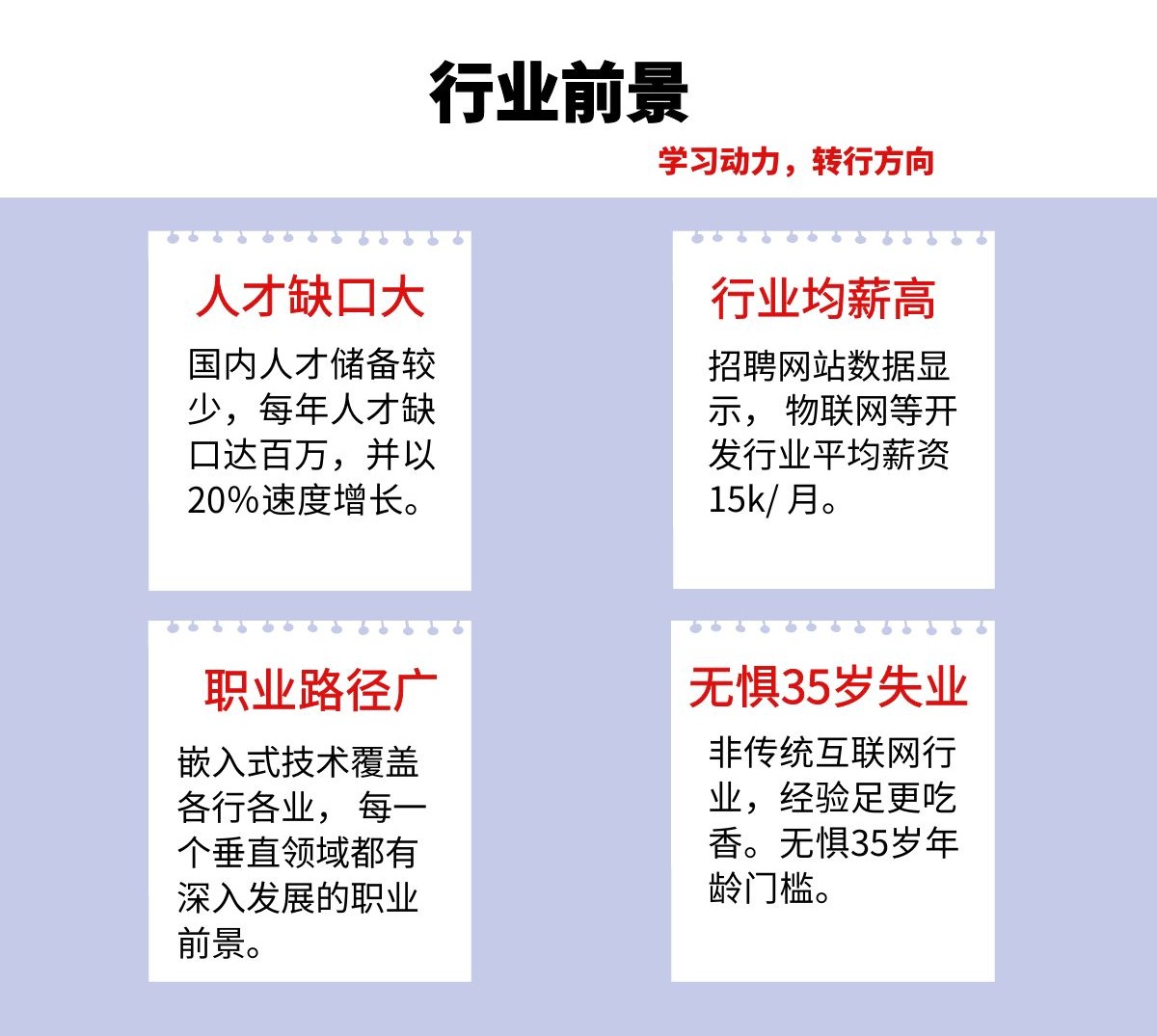
**因此收集整理了一份《2024年嵌入式&物联网开发全套学习资料》，初衷也很简单，就是希望能够帮助到想自学提升又不知道该从何学起的朋友，同时减轻大家的负担。**

![img](https://img-blog.csdnimg.cn/img_convert/3890056cb1ffb63617fd502372905143.png)

![img](https://img-blog.csdnimg.cn/img_convert/dd729f9e518920dc7baa3b2e95c8494f.jpeg)

![img](https://img-blog.csdnimg.cn/img_convert/a10bbd8e4c11b608cf5ba0a2b544df4b.png)

 ![img](https://img-blog.csdnimg.cn/img_convert/d5d5a7aad91f73dd897771ef43963c25.png)

![img](https://img-blog.csdnimg.cn/img_convert/97336336d044f3511010012b2b1cbda0.png)

![img](https://img-blog.csdnimg.cn/img_convert/00a23e0a76a2e7b701e09901adf8ace9.png)

![](https://img-blog.csdnimg.cn/img_convert/777cf5b39b2a21192a85fe8ae0beb24f.png)

 

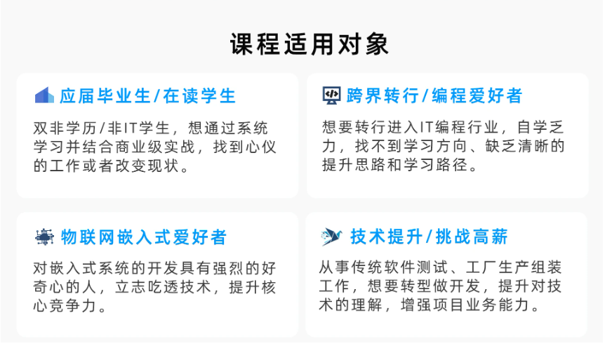
**既有适合小白学习的零基础资料，也有适合3年以上经验的小伙伴深入学习提升的进阶课程，基本涵盖了95%以上嵌入式&物联网开发知识点，真正体系化！**

[**如果你觉得这些内容对你有帮助，需要这份全套学习资料的朋友可以戳我获取！！**](https://bbs.csdn.net/topics/618654289)

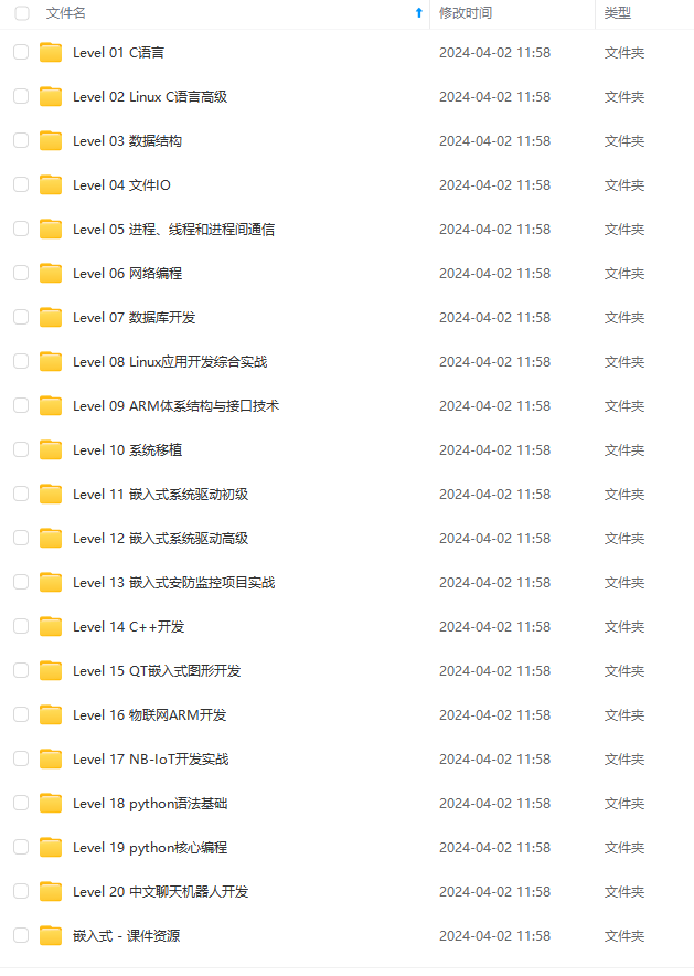
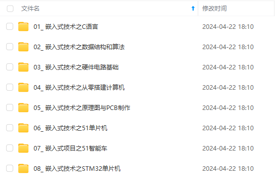
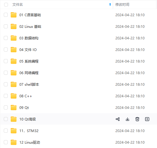
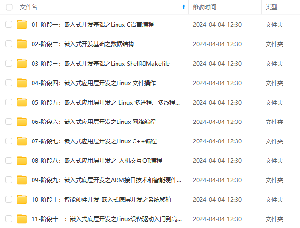
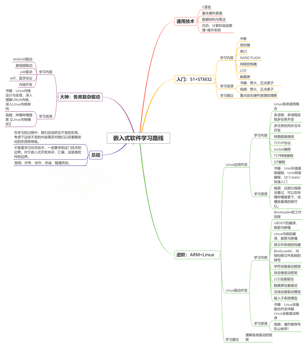
**由于文件比较大，这里只是将部分目录大纲截图出来，每个节点里面都包含大厂面经、学习笔记、源码讲义、实战项目、讲解视频，并且后续会持续更新**！！


I0-1715583993688)]

[外链图片转存中...(img-t0Q4hrO9-1715583993689)]

[外链图片转存中...(img-8I2UY0ne-1715583993689)]

 

**既有适合小白学习的零基础资料，也有适合3年以上经验的小伙伴深入学习提升的进阶课程，基本涵盖了95%以上嵌入式&物联网开发知识点，真正体系化！**

[**如果你觉得这些内容对你有帮助，需要这份全套学习资料的朋友可以戳我获取！！**](https://bbs.csdn.net/topics/618654289)

**由于文件比较大，这里只是将部分目录大纲截图出来，每个节点里面都包含大厂面经、学习笔记、源码讲义、实战项目、讲解视频，并且后续会持续更新**！！
2401_83703951
关注
3
点赞
踩
0

收藏

觉得还不错? 一键收藏
0
评论
iotdb分段分组聚合_iotdb 聚合统计

由于用户指定了滑动步长为2mo，GROUP BY 语句执行时将会每次把时间间隔往后移动 2 个自然月的步长，而不是默认的 1 个自然月。也就意味着，我们想要取从 2017-11-01 到 2019-11-07 每 2 个自然月的第一个月的数据。#按照自然月份的时间区间分组聚合查询。
复制链接

扫一扫