


早停策略和模型权重的保存
一、模型的保存和加载
深度学习中模型的保存与加载主要涉及参数(权重)和整个模型结构的存储,同时需兼顾训练状态(如优化器参数、轮次等)以支持断点续训。
仅保存模型参数(推荐)
- 原理:保存模型的权重参数,不保存模型结构代码。加载时需提前定义与训练时一致的模型类。
-
优点:文件体积小(仅含参数),跨框架兼容性强(需自行定义模型结构)。
# 保存模型参数
torch.save(model.state_dict(), "model_weights.pth")
# 加载参数(需先定义模型结构)
model = MLP()  # 初始化与训练时相同的模型结构
model.load_state_dict(torch.load("model_weights.pth"))
# model.eval()  # 切换至推理模式(可选)
保存模型+权重
- 原理:保存模型结构及参数
- 优点:加载时无需提前定义模型类
- 缺点:文件体积大,依赖训练时的代码环境(如自定义层可能报错)。
# 保存整个模型
torch.save(model, "full_model.pth")

# 加载模型(无需提前定义类,但需确保环境一致)
model = torch.load("full_model.pth")
# model.eval()  # 切换至推理模式(可选)
二、早停法
我们梳理下过拟合的情况
-
正常情况:训练集和测试集损失同步下降,最终趋于稳定。
-
过拟合:训练集损失持续下降,但测试集损失在某一时刻开始上升(或不再下降)。
如果可以监控验证集的指标不再变好,此时提前终止训练,避免模型对训练集过度拟合。监控的对象是验证集的指标。这种策略叫早停法。
# ===== 早停相关参数 =====
best_test_loss = float('inf')  # 记录最佳测试集损失
best_epoch = 0                 # 记录最佳epoch
patience = 50                # 早停耐心值(连续多少轮测试集损失未改善时停止训练)
counter = 0                    # 早停计数器
early_stopped = False          # 是否早停标志

# ===== 新增早停逻辑 =====
            if test_loss.item() < best_test_loss: # 如果当前测试集损失小于最佳损失
                best_test_loss = test_loss.item() # 更新最佳损失
                best_epoch = epoch + 1 # 更新最佳epoch
                counter = 0 # 重置计数器
                # 保存最佳模型
                torch.save(model.state_dict(), 'best_model.pth')
            else:
                counter += 1
                if counter >= patience:
                    print(f"早停触发!在第{epoch+1}轮,测试集损失已有{patience}轮未改善。")
                    print(f"最佳测试集损失出现在第{best_epoch}轮,损失值为{best_test_loss:.4f}")
                    early_stopped = True
                    break  # 终止训练循环
早停策略的具体逻辑如下:
- 首先初始一个计数器counter。
- 每 200 轮训练执行一次判断:比较当前损失与历史最佳损失。
- 若当前损失更低,保存模型参数。
- 若当前损失更高或相等,计数器加 1。
- 若计数器达到最大容许的阈值patience,则停止训练。
以信贷风险预测的数据集为例:
# 导入相关库
import pandas as pd
import numpy as np
import matplotlib.pyplot as plt
from sklearn.model_selection import train_test_split
from sklearn.preprocessing import StandardScaler, LabelEncoder, OneHotEncoder, MinMaxScaler
import torch
import torch.nn as nn
import torch.optim as optim
import seaborn as sns
import warnings
warnings.filterwarnings("ignore")
import time
# 设置GPU设备
device = torch.device("cuda:0" if torch.cuda.is_available() else "cpu")
print(f"Using device: {device}")
# 读取数据
data = pd.read_csv('data.csv')
# 查看数据
data.head()
data.info()
# 数据预处理
# 删除无用列
data.drop(columns=['Id'], inplace=True)
# 分离连续特征与离散特征
continuous_features = data.select_dtypes(include=['float64', 'int64']).columns.tolist()
discrete_features = data.select_dtypes(exclude=['float64', 'int64']).columns.tolist()
# 查看缺失值
data.isnull().sum()
# 缺失值处理
# 对于连续特征,使用中位数填充
for feature in continuous_features:
    if data[feature].isnull().sum() > 0:
        data[feature].fillna(data[feature].median(), inplace=True)
# 对于离散特征,使用众数填充
for feature in discrete_features:
    if data[feature].isnull().sum() > 0:
        data[feature].fillna(data[feature].mode()[0], inplace=True)
# 再次查看缺失值
data.isnull().sum()
# 有序离散变量进行标签编码
mappings = {
    "Years in current job": {
        "10+ years": 10,
        "2 years": 2,
        "3 years": 3,
        "< 1 year": 0,
        "5 years": 5,
        "1 year": 1,
        "4 years": 4,
        "6 years": 6,
        "7 years": 7,
        "8 years": 8,
        "9 years": 9
    },
    "Home Ownership": {
        "Home Mortgage": 0,
        "Rent": 1,
        "Own Home": 2,
        "Have Mortgage": 3
    },
    "Term": {
        "Short Term": 0,
        "Long Term": 1
    }
}
# 使用映射字典进行转换
data["Years in current job"] = data["Years in current job"].map(mappings["Years in current job"])
data["Home Ownership"] = data["Home Ownership"].map(mappings["Home Ownership"])
data["Term"] = data["Term"].map(mappings["Term"])
# 对无序离散变量进行独热编码
data = pd.get_dummies(data, columns=['Purpose'])
# 独热编码后会新增一些列,需要将这些列的类型转换为int
data2 = pd.read_csv("data.csv") # 重新读取数据,用来做列名对比
list_final = [] # 新建一个空列表,用于存放独热编码后新增的特征名
for i in data.columns:
    if i not in data2.columns:
       list_final.append(i) # 这里打印出来的就是独热编码后的特征名
for i in list_final:
    data[i] = data[i].astype(int) # 这里的i就是独热编码后的特征名
# 分离特征和标签
x = data.drop(['Credit Default'], axis=1)
y = data['Credit Default']
# 划分训练集(80%)和测试集(20%):训练集用来学习,测试集验证效果
x_train, x_test, y_train, y_test = train_test_split(x, y, test_size=0.2, random_state=42)
# 特征数据归一化处理,神经网络对于输入数据的尺寸敏感,归一化是最常见的处理方式
scaler = MinMaxScaler()
x_train = scaler.fit_transform(x_train)
x_test = scaler.transform(x_test)
# 将数据转换为PyTorch张量并移至GPU
# 分类问题交叉熵损失要求标签为long类型
# 张量具有to(device)方法,可以将张量移动到指定的设备上
x_train = torch.FloatTensor(x_train).to(device)
y_train = torch.LongTensor(y_train.values).to(device)  # 注意这里需要使用values属性
x_test = torch.FloatTensor(x_test).to(device)
y_test = torch.LongTensor(y_test.values).to(device)
# 打印下尺寸
print(x_train.shape)
print(y_train.shape)
print(x_test.shape)
print(y_test.shape)

import torch.nn as nn # 导入PyTorch的神经网络模块
import torch.optim as optim # 导入PyTorch的优化器模块
class MLP(nn.Module): # 定义一个多层感知机(MLP)模型,继承父类nn.Module
    def __init__(self): # 初始化函数
        super(MLP, self).__init__() # 调用父类的初始化函数
 # 定义的前三行是八股文,后面的是自定义的
        self.fc1 = nn.Linear(30, 64) # 首隐藏层建议为输入层的2-4倍
        self.relu = nn.ReLU() # 定义激活函数ReLU
        self.fc2 = nn.Linear(64, 2) # 定义第二个全连接层,输入维度为10,输出维度为3
# 输出层不需要激活函数,因为后面会用到交叉熵函数cross_entropy,交叉熵函数内部有softmax函数,会把输出转化为概率
    def forward(self, x):
        out = self.fc1(x) # 输入x经过第一个全连接层
        out = self.relu(out) # 激活函数ReLU
        out = self.fc2(out) # 输入out经过第二个全连接层
        return out # 返回输出

# 实例化模型
model = MLP().to(device) # 将模型移至GPU

class MLP(nn.Module):
    def __init__(self):
        super(MLP, self).__init__()
        self.fc1 = nn.Linear(30, 64)  # 输入层到第一隐藏层
        self.relu = nn.ReLU()  # 激活函数ReLU
        self.dropout = nn.Dropout(0.3)  # 添加Dropout防止过拟合
        self.fc2 = nn.Linear(64, 32)  # 第一隐藏层到第二隐藏层
        self.fc3 = nn.Linear(32, 2)  # 第二隐藏层到输出层

    def forward(self, x):
        x = self.fc1(x)
        x = self.relu(x)
        x = self.dropout(x)
        x = self.fc2(x)
        x = self.relu(x)
        x = self.dropout(x)
        x = self.fc3(x)
        return x

# 初始化模型
model = MLP().to(device)
# 定义损失函数和优化器
# 分类问题使用交叉熵损失函数,适用于多分类问题,应用softmax函数将输出映射到概率分布,然后计算交叉熵损失
criterion = nn.CrossEntropyLoss()
# 使用随机梯度下降优化器(SGD),学习率为0.01
optimizer = optim.SGD(model.parameters(), lr=0.01)


# 训练模型
num_epochs = 20000  # 训练的轮数
# 用于存储每200个epoch的损失值和对应的epoch数
train_losses = []  # 存储训练集损失
test_losses = []   # 存储测试集损失
epochs = []

# ===== 新增早停相关参数 =====
best_test_loss = float('inf')  # 记录最佳测试集损失
best_epoch = 0                 # 记录最佳epoch
patience = 50                # 早停耐心值(连续多少轮测试集损失未改善时停止训练)
counter = 0                    # 早停计数器
early_stopped = False          # 是否早停标志
# ==========================
from tqdm import tqdm  # 导入tqdm库用于进度条显示
start_time = time.time()  # 记录开始时间
# 创建tqdm进度条
with tqdm(total=num_epochs, desc="训练进度", unit="epoch") as pbar:
    # 训练模型
    for epoch in range(num_epochs):
        # 前向传播
        outputs = model(x_train)  # 模型预测输出
        train_loss = criterion(outputs, y_train) # 计算损失

        # 反向传播和优化
        optimizer.zero_grad()  # 清空梯度
        train_loss.backward()  # 反向传播
        optimizer.step()  # 更新参数

        # 记录损失值并更新进度条
        if (epoch + 1) % 200 == 0:
            # 计算测试集损失
            model.eval()  # 设置模型为评估模式
            with torch.no_grad():  # 关闭梯度计算
                test_outputs = model(x_test) # 测试集预测输出
                test_loss = criterion(test_outputs, y_test) # 计算测试集损失
            model.train()
            # 记录损失值和epoch数
            train_losses.append(train_loss.item())
            test_losses.append(test_loss.item())
            epochs.append(epoch + 1)

            # 更新进度条的描述信息
            pbar.set_postfix({'Train Loss': f'{train_loss.item():.4f}', 'Test Loss': f'{test_loss.item():.4f}'})

            # ===== 新增早停逻辑 =====
            if test_loss.item() < best_test_loss: # 如果当前测试集损失小于最佳损失
                best_test_loss = test_loss.item() # 更新最佳损失
                best_epoch = epoch + 1 # 更新最佳epoch
                counter = 0 # 重置计数器
                # 保存最佳模型
                torch.save(model.state_dict(), 'best_model.pth')
            else:
                counter += 1
                if counter >= patience:
                    print(f"早停触发!在第{epoch+1}轮,测试集损失已有{patience}轮未改善。")
                    print(f"最佳测试集损失出现在第{best_epoch}轮,损失值为{best_test_loss:.4f}")
                    early_stopped = True
                    break  # 终止训练循环
            # ======================

        # 每1000个epoch更新一次进度条
        if (epoch + 1) % 1000 == 0:
            pbar.update(1000)  # 更新进度条

    # 确保进度条达到100%
    if pbar.n < num_epochs:
        pbar.update(num_epochs - pbar.n)  # 计算剩余的进度并更新

time_all = time.time() - start_time  # 计算训练时间
print(f'Training time: {time_all:.2f} seconds')

# ===== 新增:加载最佳模型用于最终评估 =====
if early_stopped:
    print(f"加载第{best_epoch}轮的最佳模型进行最终评估...")
    model.load_state_dict(torch.load('best_model.pth'))

    # ===== 新增继续训练逻辑 =====
    print(f"加载第{best_epoch}轮的最佳模型继续训练50轮...")
    model.load_state_dict(torch.load('best_model.pth'))

    # 重置早停参数
    best_test_loss = float('inf')
    counter = 0
    early_stopped = False

    # 继续训练50轮
    with tqdm(total=50, desc="继续训练进度", unit="epoch") as cont_pbar:
        for epoch in range(50):
            outputs = model(x_train)
            train_loss = criterion(outputs, y_train)

            optimizer.zero_grad()
            train_loss.backward()
            optimizer.step()

            # 每10轮评估一次
            if (epoch + 1) % 10 == 0:
                model.eval()
                with torch.no_grad():
                    test_outputs = model(x_test)
                    test_loss = criterion(test_outputs, y_test)
                model.train()

                # 更新早停逻辑
                if test_loss.item() < best_test_loss:
                    best_test_loss = test_loss.item()
                    counter = 0
                    torch.save(model.state_dict(), 'best_model.pth')
                else:
                    counter += 1
                    if counter >= patience:
                        print(f"继续训练中触发早停!")
                        break

            cont_pbar.update(1)

# 可视化损失曲线
plt.figure(figsize=(10, 6))
plt.plot(epochs, train_losses, label='Train Loss')
plt.plot(epochs, test_losses, label='Test Loss')
plt.xlabel('Epoch')
plt.ylabel('Loss')
plt.title('Training and Test Loss over Epochs')
plt.legend()
plt.grid(True)
plt.show()

# 在测试集上评估模型
model.eval()
with torch.no_grad():
    outputs = model(x_test)  # 模型预测
    _, predicted = torch.max(outputs, 1)
    correct = (predicted == y_test).sum().item()
    accuracy = correct / y_test.size(0)
print(f'测试集准确率: {accuracy * 100:.2f}%') 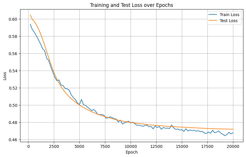
得到测试集准确率:76.87%
之所以设置阈值patience,是因为训练过程中存在波动,不能完全停止训练。同时每隔固定的训练轮次都会保存模型参数,下次可以接着这里训练,缩小训练的范围。
这里之所以没有触发早停策略,有以下几个原因:
- 测试集损失在训练中持续下降或震荡,但未出现连续 patience 轮不改善
- patience值过大,需要调小
实际上,在早停策略中,保存 checkpoint(检查点) 是更优选择,因为它不仅保存了模型参数,还记录了训练状态(如优化器参数、轮次、损失值等),一但出现了过拟合,方便后续继续训练


 被折叠的 条评论
为什么被折叠?
被折叠的 条评论
为什么被折叠?
 到【灌水乐园】发言


