二叉树学习笔记-CSDN博客

本文链接：https://blog.csdn.net/BlueDre/article/details/140701412

二叉树学习笔记

树

在了解二叉树之前，首先要了解比二叉树更大一级的概念，不仅是为了在学习二叉树的时候不至于不明白这两个具有包含关系的两个事物的相同之处，还是为了能够在有一个更为宏观的认知，不至于管中窥豹。

树的概念

树是一种非线性的数据结构，它是由n（n>=0）个有限结点组成一个具有层次关系的集合。

一些概念：

**节点的度：**一个节点含有的子树的个数
**叶节点：**度为0的节点
**分支节点：**度不为0的节点
**父节点：**含有子节点的节点
**子节点：**子树的根节点
**兄弟节点：**具有相同父节点的节点
**树的度：**最大的节点的度
**节点的层次：**从根开始定义，从1开始数起
**树的高度：**树中节点的最大层次
**节点的祖先：**从该节点往上分支的所有节点
**子孙：**以某结点为根的子树中任一结点都称为该结点的子孙
**森林：**互不相交的树的集合称为森林

树的表示方法

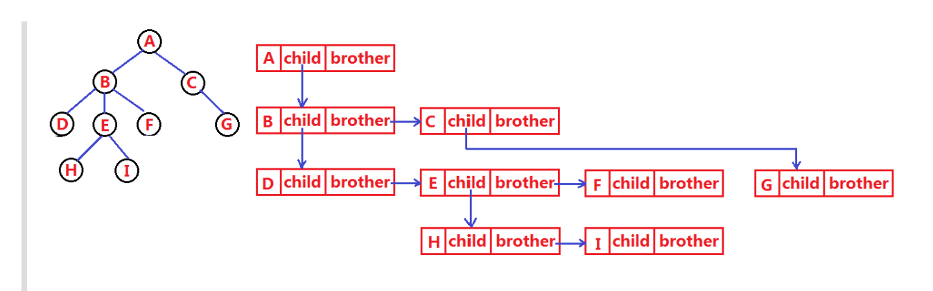
为了清楚保存节点之间的关系，可以采用孩子兄弟表示法，具体是这么做的：

保存指向第一个子节点的指针
保存指向右边第一个兄弟节点的指针

如图

其实现代码如下：

typedef int DataType;
struct Node{
    struct Node* FirstChild;
    struct Node* NextBrother;
    DataType data;
}

二叉树

在了解完树以后，在了解二叉树就更容易了，首先来看看定义：

一棵二叉树是结点的一个有限集合，该集合可以为空，也可以由一个根节点加上两棵别称为左子树和右子树的二叉树组成。

特殊的二叉树

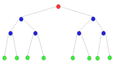
满二叉树：一颗二叉树，除最后一层外每个节点都有二个子节点，也就是在二叉树的基础上，即每个节点最大只有两个子节点，同时满足这个最大条件，如图：
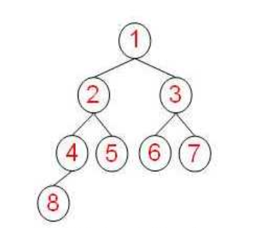
完全二叉树：完全二叉树是由满二叉树而引出来，相比于满二叉树，完全二叉树最后一层不一定是满的，并且最后一层的节点从左至右依次排布，也可以认为满二叉树是其特殊情况，如图：

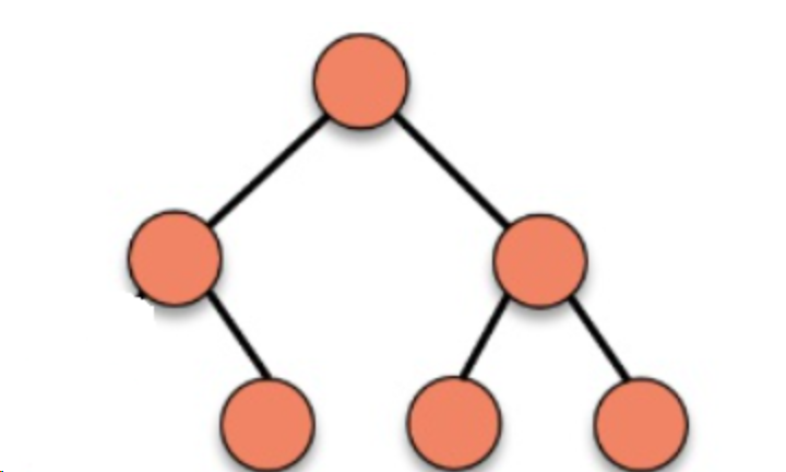
像这样的就不是完全二叉树，没有左排列：

二叉树的性质

二叉树不是无缘无故想出来的，是为了作为数据结构，既然树是一种非线性的数据结构，那么我们的储存和查找

就要根据其性质来进行。

深度为h的二叉树的最大结点数是 $2^h-1$
一棵非空二叉树的第i层上最多有 $2^{i-1}$ 个结点
n个结点的满二叉树的深度, $h=\log_2(n+1)$

堆

以完全二叉树为逻辑顺序所建立的数据结构叫做堆，堆有大堆和小堆之分，在大堆中，父节点大于其子节点，同样的，在小堆中，父节点小于其子节点。

堆的实现

引用及声明

#include <stdlib.h>
#include <assert.h>
#include <stdio.h>
typedef int HPDataType;
typedef struct Heap
{
	HPDataType* _a;
	int _size;
	int _capacity;
}Heap;

void HeapInit(Heap* php);
// 堆的销毁
void HeapDestory(Heap* hp);
// 堆的插入
void HeapPush(Heap* hp, HPDataType x);
// 堆的删除
void HeapPop(Heap* hp);
// 取堆顶的数据
HPDataType HeapTop(Heap* hp);
// 堆的数据个数
int HeapSize(Heap* hp);
// 堆的判空
int HeapEmpty(Heap* hp);

函数实现

void Swap(HPDataType* A, HPDataType* B)
{
	HPDataType tmp = *A;
	*A = *B;
	*B = tmp;
}

void AdjustUp(HPDataType* arr, int child) {
	
	int parrent = (child - 1) / 2;
	while (child > 0) {
		//小堆的情况下
		if (arr[child] < arr[parrent]) {
			Swap(&arr[child], &arr[parrent]);
			child = parrent;
			parrent = (child - 1) / 2;
		}
		else {
			break;
		}
	}
}

void AdjustDown(HPDataType* arr, int n, int parent) {
	//小堆的情况
	int child = parent * 2 + 1;
	while (child < n) {
		if (arr[child] > arr[child + 1] && child + 1 < n) {
			child++;
		}
		if (arr[child] < arr[parent]) {
			Swap(&arr[child], &arr[parent]);
			parent = child;
			child = parent * 2 + 1;
		}
		else {
			break;
		}

	}
	
}

void HeapInit(Heap* php) {
	assert(php);
	php->_a = NULL;
	php->_capacity = php->_size = 0;

}

void HeapDestory(Heap* hp) {
	assert(hp);
	free(hp->_a);
	hp->_a = NULL;
	hp->_capacity = hp->_size = 0;

}

void HeapPush(Heap* hp, HPDataType x) {
	assert(hp);
	if (hp->_capacity == hp->_size) {
		int Newcapacity = hp->_capacity == 0 ? 4 : hp->_capacity * 2;
		HPDataType* tmp = (HPDataType*)realloc(hp->_a, Newcapacity * sizeof(HPDataType));
		if (tmp == NULL) {
			perror("realloc fail");
			exit(1);
		}
		hp->_a = tmp;
		hp->_capacity = Newcapacity;
	}
	hp->_a[hp->_size] = x;
	hp->_size++;
	AdjustUp(hp->_a, hp->_size - 1);
}

void HeapPop(Heap* hp) {
	assert(hp);
	assert(hp->_size > 0);
	Swap(&hp->_a[0], &hp->_a[hp->_size-1]);
	hp->_size--;
	AdjustDown(hp->_a, hp->_size, 0);
}

HPDataType HeapTop(Heap* hp) {
	assert(hp);
	assert(hp->_size > 0);
	return hp->_a[0];
}
int HeapSize(Heap* hp) {
	assert(hp);
	return hp->_size;
}
int HeapEmpty(Heap* hp) {
	assert(hp);
	if (hp->_size != 0)return 0;
	else return -1;
}

堆排序

堆排序的实现

到目前已经创建了堆这样的数据结构，可以用它来进行排序的操作。不过非线性的数据结构该怎么来排序呢？根据大小堆的性质进行实现。其算法可以分为三步：

将原本散乱的数据根据升序要求和降序要求分别建立大堆和小堆
将堆顶和堆的最后一个叶子进行交换
进行范围缩小的堆调整使堆恢复

实现代码如下：

void HeapSort(int* arr, int n) {
	//降序排列 小堆
	//向上调整法 
	//for (int i = 1; i < n; i++) {
	//	AdjustUp(arr, i);
	//}
	//向下调整法建堆
	for (int i = (n - 1 - 1) / 2; i >= 0; i--) {
		AdjustDown(arr, n, i);
	}
    
	int end = n - 1;
	while (end>0) {
		Swap(&arr[0], &arr[end]);
		AdjustDown(arr, end, 0);
		end--;
	}
}

可以看到，在第一步中，出现了两种算法，一种是向上调整法，另一种是向下调整法，使用向下调整法则效率更高，推导如下：

向下调整算法

$树的高度：h=\log_2(N+1)\\ 每一层的节点数：n=2^{i-1}\\ 总节点数为：n=2^h-1\\ 则向下调整的总深度为：T(N)=2^{h-2}*1 + 2^{h-3}*2 + ... + 2^0*(h-1)\\ 利用错位相减法可得：2T(N)=2^{h-1}*1 + 2^{h-2}*2 + ... + 2^1*(h-1)\\ T(N)=2^{h-1}+2^{h-2}+...+2^1-(h-1)=2^h-1-h\\ 将n带入可得：O(n)= n-\log_2(n+1)=n$

向上调整算法

$树的高度：h=\log_2(N+1)\\ 每一层的节点数：n=2^{i-1}\\ 总节点数为：n=2^h-1\\ 则向上调整的总深度为：T(N)=2^{h-1}*(h-1) + 2^{h-2}*(h-2) + ... 2^1*1\\ 利用错位相减法可得：2T(N)=2^{h}*(h-1) + 2^{h-1}*(h-2) + ... + 2^2*(h-1)\\ T(N)=h*2^h-2\\ 将n带入可得：O(n)= (n+1)\log_2(n+1)=n\log n$

堆排序的应用

Top k问题：Top k问题指的是求一组数中前k个数的问题，可能是求最大的前k个数，也可能是最小的前k个数。

利用堆排序来解决这一类问题，其优势在于他的时间复杂度只有 $O(n\log n)$ ,以及在数据量大的情况下它仍能够使用，这里讲述数据量大时的处理方法。

建造一个对应的大小为k的堆
将堆顶与未进入堆的数进行对比，根据需求条件进行堆顶的替换
进行向下调整
重复2和3

二叉树的实现

二叉树的遍历

前序遍历

void BinaryTreePrevOrder(BTNode* root) {
	if (root == NULL) {
		return;
	}
	printf("%c", root->_data);
	BinaryTreePrevOrder(root->_left);
	BinaryTreePrevOrder(root->_right);
}

中序遍历

void BinaryTreeInOrder(BTNode* root) {
	if (root == NULL) {
		return;
	}
	BinaryTreeInOrder(root->_left);
	printf("%c", root->_data);
	BinaryTreeInOrder(root->_right);
}

后序遍历

void BinaryTreePostOrder(BTNode* root) {
	if (root == NULL) {
		return;
	}
	BinaryTreePostOrder(root->_left);
	BinaryTreePostOrder(root->_right);
	printf("%c", root->_data);
}

层序遍历

void BinaryTreeLevelOrder(BTNode* root) {
	Queue q;
	QueueInit(&q);
	if (root)
		QueuePush(root, &q);

	while (!QueueEmpty(&q))
	{
		BTNode* front = QueueFront(&q);
		QueuePop(&q);
		printf("%d ", front->_data);

		if (front->_left)
			QueuePush(&q,front->_left);
		if (front->_right)
			QueuePush(&q,front->_right);

	}

	QueueDestroy(&q);
}

树的创建和销毁

通过前序遍历的数组构建二叉树

BTNode* BinaryTreeCreate(BTDataType* a, int n, int* pi) {
	if (*pi >= n) {
		return NULL;
	}

	if (a[*pi] == '#') {
		(*pi)++;
		return NULL;
	}
	BTNode* root = (BTNode*)malloc(sizeof(BTNode));
	root->_data = a[(*pi)++];
	root->_left=BinaryTreeCreate(a, n, pi);
	root->_right = BinaryTreeCreate(a, n, pi);
	return root;

}

二叉树销毁

void BinaryTreeDestory(BTNode** root) {
	if (*root == NULL) {
		return;
	}
	if ((*root)->_left != NULL) {
		BTNode** root_left = &((*root)->_left);
		BinaryTreeDestory(root_left);
		free(*root);
		return;
	}
	if ((*root)->_right != NULL) {
		BTNode** root_right = &((*root)->_right);
		BinaryTreeDestory(root_right);
		free(*root);
		return;
	}	

}

二叉树应用

二叉树节点个数

int BinaryTreeSize(BTNode* root) {
	if (root == NULL) {
		return 0;
	}

	int size = BinaryTreeSize(root->_left) + BinaryTreeSize(root->_right);

	return size+1;
}

二叉树叶子节点个数

int BinaryTreeLeafSize(BTNode* root) {
	if (root == NULL) {
		return 0;
	}

	if (root->_left == NULL && root->_right == NULL) {
		return 1;
	}
	int size = BinaryTreeLeafSize(root->_left) + BinaryTreeLeafSize(root->_right);
	return size;
}

二叉树第k层节点个数

int BinaryTreeLevelKSize(BTNode* root, int k) {

	if (root == NULL) {
		return 0;
	}

	if (k==1 && root != NULL) {
		return 1;
	}
	int size = BinaryTreeLevelKSize(root->_left,k-1) + BinaryTreeLevelKSize(root->_right,k-1);

	return size;
}

二叉树查找值为x的节点

int BinaryTreeLevelKSize(BTNode* root, int k) {

	if (root == NULL) {
		return 0;
	}

	if (k==1 && root != NULL) {
		return 1;
	}
	int size = BinaryTreeLevelKSize(root->_left,k-1) + BinaryTreeLevelKSize(root->_right,k-1);

	return size;
}

判断二叉树是否是完全二叉树

int BinaryTreeComplete(BTNode* root) {
	Queue q;
	QueueInit(&q);
	if (root)
		QueuePush(root, &q);

	
	while (!QueueEmpty(&q)) {
		BTNode* front = QueueFront(&q);
		QueuePop(&q);
		if (front == NULL) {
			break;
		}

		QueuePush(&q, front->_left);
		QueuePush(&q, front->_right);
	}

	while (!QueueEmpty(&q)) {
		BTNode* front = QueueFront(&q);
		QueuePop(&q);
		if (front != NULL) {
			QueueDestroy(&q);
			return 0;
		}


	}
	QueueDestroy(&q);
	return 1;

}

一些重点

递归的使用：

三大项：

定义函数功能
寻找结束条件
递推函数的等价关系

注意事项：

对函数结果进行记录避免多次调用

对任何一棵二叉树, 如果度为0其叶结点个数为 $n_0$ , 度为2的分支结点个数为 $n_2$ ,则有 $n_0$ ＝ $n_2$ ＋1

关系推导：

要增加度为1的节点，则度为0的节点转化为度为1的节点

要增加度为2的节点，则度为1的节点转化为度为2的节点

即要获得一个度为2的节点，要对同一节点进行两次增加操作，第一次增加时久的度为0的节点转化为度为1，新的度为0节点生成，第二次增加时度为1的节点转化为度为2，度为0的节点+1，则每个 $n_2$ 节点的生成都需要2个 $n_0$ ，即 $n_0$ ＝ $n_2$ ＋1

已知遍历结果倒推二叉树

已知两种结果求另外一个结果:

分为两大步骤：
1. 确定根节点
2. 确定左右子树
已知节点个数求二叉树种类个数
1. 利用卡特兰数进行计算：
  $C_n=\frac {(2n)!}{(n+1)!n!}$
2. 利用递归关系式：
  $C_n=\sum_{i=0}^{n-1}C_i*C_{n-1-i}$