用tensorflow做一元线性回归

import numpy as np
import matplotlib.pyplot as plt
import os
import tensorflow as tf
os.environ['TF_CPP_MIN_LOG_LEVEL'] = '2'

# 产生训练数据集
train_X = np.asarray([3.3,4.4,5.5,6.71,6.93,4.168,9.779,6.182,7.59,2.167,
                         7.042,10.791,5.313,7.997,5.654,9.27,3.1])
train_Y = np.asarray([1.7,2.76,2.09,3.19,1.694,1.573,3.366,2.596,2.53,1.221,
                         2.827,3.465,1.65,2.904,2.42,2.94,1.3])
n_train_samples = train_X.shape[0]
print('训练样本数量: ', n_train_samples)
# 产生测试样本
test_X = np.asarray([6.83, 4.668, 8.9, 7.91, 5.7, 8.7, 3.1, 2.1])
test_Y = np.asarray([1.84, 2.273, 3.2, 2.831, 2.92, 3.24, 1.35, 1.03])
n_test_samples = test_X.shape[0]
print('测试样本数量: ', n_test_samples)

# 展示原始数据分布
plt.plot(train_X, train_Y, 'ro', label='Original Train Points')
plt.plot(test_X, test_Y, 'b*', label='Original Test Points')
plt.legend()
plt.show()

print('~~~~~~~~~~开始设计计算图~~~~~~~~')
# 告诉TensorFlow模型将会被构建在默认的Graph上.
with tf.Graph().as_default():
    # Input: 定义输入节点
    with tf.name_scope('Input'):
        # 计算图输入占位符
        X = tf.placeholder(tf.float32, name='X')
        Y_true = tf.placeholder(tf.float32, name='Y_true')
    # Inference: 定义预测节点
    with tf.name_scope('Inference'):
        # 回归模型的权重和偏置
        # np.random.randn()返回一个标准正态分布随机数
        W = tf.Variable(np.random.randn(), name="Weight")
        b = tf.Variable(np.random.randn(), name="Bias")
        # inference: 创建一个线性模型：y = wx + b
        Y_pred = tf.add(tf.multiply(X,W), b)
    #Loss: 定义损失节点
    with tf.name_scope('Loss'):
        TrainLoss = tf.reduce_mean(tf.pow((Y_pred - Y_true), 2))/2
    # Train: 定义训练节点
    with tf.name_scope('Train'):
        # Optimizer: 创建一个梯度下降优化器
        Optimizer = tf.train.GradientDescentOptimizer(learning_rate=0.01)
        # Train: 定义训练节点将梯度下降法应用于Loss
        TrainOp = Optimizer.minimize(TrainLoss)
    # Evaluate: 定义评估节点
    with tf.name_scope('Evaluate'):
        # Loss = tf.reduce_sum(tf.pow((Y_pred-Y_true), 2))/(2*n_test_samples)
        EvalLoss = tf.reduce_mean(tf.pow((Y_pred - Y_true), 2)) / 2
    #Initial:添加所有Variable类型的变量的初始化节点
    InitOp = tf.global_variables_initializer()

    print('把计算图写入事件文件，在TensorBoard里面查看')
    writer = tf.summary.FileWriter(logdir='logs', graph=tf.get_default_graph())
    writer.close()

    print('启动会话，开启训练评估模式，让计算图跑起来')
    sess = tf.Session()
    sess.run(InitOp)  #运行初始化节点，完成初始化

    print("不断的迭代训练并测试模型")
    for step in range(1000):
        _, train_loss, train_w, train_b = sess.run([TrainOp, TrainLoss, W, b],
                                                   feed_dict={X: train_X, Y_true: train_Y})
        # 每隔几步训练完之后输出当前模型的损失
        if (step + 1) % 50 == 0:
            print("Step:", '%04d' % (step + 1), "train_loss=", "{:.9f}".format(train_loss),
                  "W=", train_w, "b=", train_b)

        # 每隔几步训练完之后对当前模型进行测试
        if (step + 1) % 50 == 0:
            test_loss, test_w, test_b = sess.run([EvalLoss, W, b],
                                                 feed_dict={X: test_X, Y_true: test_Y})
            print("Step:", '%04d' % (step + 1), "test_loss=", "{:.9f}".format(test_loss),
                  "W=", test_w, "b=", test_b)

    print("训练结束!")
    W, b = sess.run([W, b])
    print("得到的模型参数：", "W=", W, "b=", b,)
    training_loss = sess.run(TrainLoss, feed_dict={X: train_X, Y_true: train_Y})
    print("训练集上的损失：", training_loss)
    test_loss = sess.run(EvalLoss, feed_dict={X: test_X, Y_true: test_Y})
    print("测试集上的损失：", test_loss)
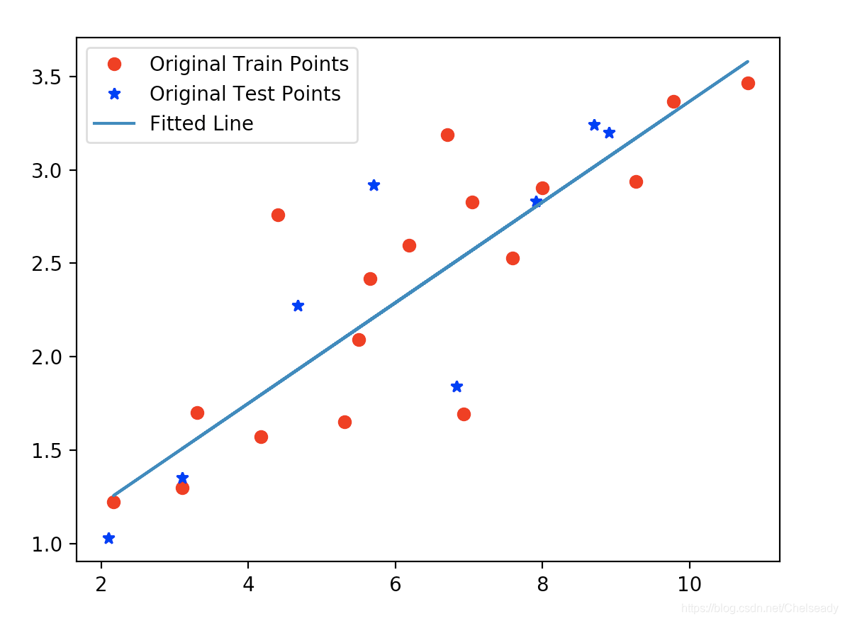
    # 展示拟合曲线
    plt.plot(train_X, train_Y, 'ro', label='Original Train Points')
    plt.plot(test_X, test_Y, 'b*', label='Original Test Points')
    plt.plot(train_X, W * train_X + b, label='Fitted Line')
    plt.legend()
    plt.show()

运行结果：

 

训练样本数量:  17
测试样本数量:  8
~~~~~~~~~~开始设计计算图~~~~~~~~
把计算图写入事件文件，在TensorBoard里面查看
启动会话，开启训练评估模式，让计算图跑起来
不断的迭代训练并测试模型
Step: 0050 train_loss= 0.086927824 W= 0.308258 b= 0.397372
Step: 0050 test_loss= 0.077852197 W= 0.308258 b= 0.397372
Step: 0100 train_loss= 0.085784219 W= 0.304921 b= 0.421025
Step: 0100 test_loss= 0.077264316 W= 0.304921 b= 0.421025
Step: 0150 train_loss= 0.084771425 W= 0.301782 b= 0.443284
Step: 0150 test_loss= 0.076781228 W= 0.301782 b= 0.443284
Step: 0200 train_loss= 0.083874494 W= 0.298827 b= 0.464231
Step: 0200 test_loss= 0.076388791 W= 0.298827 b= 0.464231
Step: 0250 train_loss= 0.083080120 W= 0.296046 b= 0.483945
Step: 0250 test_loss= 0.076074444 W= 0.296046 b= 0.483945
Step: 0300 train_loss= 0.082376570 W= 0.29343 b= 0.502496
Step: 0300 test_loss= 0.075827442 W= 0.29343 b= 0.502496
Step: 0350 train_loss= 0.081753530 W= 0.290967 b= 0.519955
Step: 0350 test_loss= 0.075638123 W= 0.290967 b= 0.519955
Step: 0400 train_loss= 0.081201732 W= 0.288649 b= 0.536385
Step: 0400 test_loss= 0.075498156 W= 0.288649 b= 0.536385
Step: 0450 train_loss= 0.080713041 W= 0.286469 b= 0.551847
Step: 0450 test_loss= 0.075400360 W= 0.286469 b= 0.551847
Step: 0500 train_loss= 0.080280237 W= 0.284416 b= 0.566397
Step: 0500 test_loss= 0.075338274 W= 0.284416 b= 0.566397
Step: 0550 train_loss= 0.079896949 W= 0.282485 b= 0.580091
Step: 0550 test_loss= 0.075306416 W= 0.282485 b= 0.580091
Step: 0600 train_loss= 0.079557478 W= 0.280667 b= 0.592978
Step: 0600 test_loss= 0.075299934 W= 0.280667 b= 0.592978
Step: 0650 train_loss= 0.079256833 W= 0.278956 b= 0.605105
Step: 0650 test_loss= 0.075314686 W= 0.278956 b= 0.605105
Step: 0700 train_loss= 0.078990571 W= 0.277347 b= 0.616518
Step: 0700 test_loss= 0.075346984 W= 0.277347 b= 0.616518
Step: 0750 train_loss= 0.078754775 W= 0.275832 b= 0.627258
Step: 0750 test_loss= 0.075393766 W= 0.275832 b= 0.627258
Step: 0800 train_loss= 0.078545943 W= 0.274406 b= 0.637366
Step: 0800 test_loss= 0.075452246 W= 0.274406 b= 0.637366
Step: 0850 train_loss= 0.078360990 W= 0.273064 b= 0.646878
Step: 0850 test_loss= 0.075520083 W= 0.273064 b= 0.646878
Step: 0900 train_loss= 0.078197189 W= 0.271802 b= 0.655829
Step: 0900 test_loss= 0.075595260 W= 0.271802 b= 0.655829
Step: 0950 train_loss= 0.078052118 W= 0.270613 b= 0.664253
Step: 0950 test_loss= 0.075676084 W= 0.270613 b= 0.664253
Step: 1000 train_loss= 0.077923678 W= 0.269495 b= 0.672181
Step: 1000 test_loss= 0.075761035 W= 0.269495 b= 0.672181
训练结束!
得到的模型参数： W= 0.269495 b= 0.672181
训练集上的损失： 0.0779212
测试集上的损失： 0.075761