Sklearn-PolynomialFeatures()

sklearn类：

classsklearn.preprocessing.PolynomialFeatures(degree=2,interaction_only=False, include_bias=True)

专门产生多项式的，并且多项式包含的是相互影响的特征集。比如：一个输入样本是２维的。形式如[a,b] ,则二阶多项式的特征集如下[1,a,b,a^2,ab,b^2]。

• 参数解释：

degree : integer，The degree of the polynomial features. Default = 2.

多项式的阶数，一般默认是２。

interaction_only : boolean, default = False；If true,only interaction features are produced: features that are products of at mostdegree distinct input features (so not x[1] ** 2, x[0] * x[2] ** 3, etc.).

如果值为true(默认是false),则会产生相互影响的特征集。

include_bias : boolean；If True (default), then include a bias column, thefeature in which all polynomial powers are zero (i.e. a column of ones - actsas an intercept term in a linear model).

是否包含偏差列。

• 属性：

powers_ : array, shape (n_input_features,n_output_features)

powers_[i, j] is the exponent指数 of thejth input in the ith output.

n_input_features_ : int，输入特征的个数。

n_output_features_ : int，输出多项式的特征个数。它的计算是通过遍历所有的适当大小的输入特征组合。

注意：多项式的阶数不要太高，否则会出现过拟合。

• 方法：

fit(X, y=None)：计算输出特征的个数

fit_transform(X, y=None, **fit_params)：Fit todata, then transform it.

X: Training set.

y: Target values.

Returns: 

X_new: Transformed array.

get_params([deep]) :Getparameters for this estimator得到模型的参数。

set_params(**params) ：Set the parameters of this estimator.设置参数

transform(X[, y]) ：Transform data to polynomial features

• 示例：

1. 简单示例:

>>>X = np.arange(6).reshape(3, 2)
>>>X
array([[0,1],
       [2, 3],
       [4, 5]])
>>> poly =PolynomialFeatures(2)  #设置多项式阶数为２，其他的默认
>>>poly.fit_transform(X)
array([[  1.,  0.,   1.,   0.,  0.,   1.],
       [ 1.,   2.,   3.,  4.,   6.,   9.],
       [ 1.,   4.,   5., 16.,  20.,  25.]])
>>> poly =PolynomialFeatures(interaction_only=True)  #＃默认的阶数是２，同时设置交互关系为true
>>>poly.fit_transform(X)
array([[  1.,  0.,   1.,   0.],
       [ 1.,   2.,   3.,  6.],
       [ 1.,   4.,   5., 20.]])

解释：上面的数组中，每一行是一个list。比如[0,1]类似与上面的[a,b]。好的现在它的多项式输出矩阵就是[1,a,b,a^2,ab,b^2]。所以就是下面对应的[1,0,1,0,0,1]。现在将interaction_only=True。这时就是只找交互作用的多项式输出矩阵。例如[a,b]的多项式交互式输出[1,a,b,ab]。不存在自己与自己交互的情况如;a^2或者a*b^2之类的。

2. 复杂实例：

importnumpy as np
importmatplotlib.pyplot as plt
 
fromsklearn.linear_model import Ridge
fromsklearn.preprocessing import PolynomialFeatures
fromsklearn.pipeline import make_pipeline
 
deff(x):
    """ function to approximateby polynomial interpolation"""
    return x * np.sin(x)
 
#generate points used to plot
x_plot= np.linspace(0, 10, 100)
 
#generate points and keep a subset of them
x= np.linspace(0, 10, 100)
rng= np.random.RandomState(0)
rng.shuffle(x)
x= np.sort(x[:20])
y= f(x)
 
#create matrix versions of these arrays
X= x[:, np.newaxis]
X_plot= x_plot[:, np.newaxis]
 
colors= ['teal', 'yellowgreen', 'gold']
lw= 2
plt.plot(x_plot,f(x_plot), color='cornflowerblue', linewidth=lw,
         label="ground truth")
plt.scatter(x,y, color='navy', s=30, marker='o', label="training points")
 
forcount, degree in enumerate([3, 4, 5]):
    model =make_pipeline(PolynomialFeatures(degree), Ridge())
    model.fit(X, y)
    y_plot = model.predict(X_plot)
    plt.plot(x_plot, y_plot,color=colors[count], linewidth=lw,
             label="degree %d" %degree)
 
plt.legend(loc='lowerleft')
 
plt.show()

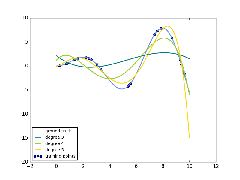
解释：这个例子是示范如何通过岭回归使用一个多项式来近似一个函数。具体的说就是不从n个输入特征的第一个特征开始，它是能够构建一个范德蒙矩阵，故n个输入特征构成的范德蒙矩阵如下：

[[1,x_1, x_1 ** 2, x_1 ** 3, ...],

[1,x_2, x_2 ** 2, x_2 ** 3, ...], ...]

直观地说，这个矩阵可以被解释为一个伪特征矩阵。这个矩阵就类似于由多项式内核产生的矩阵。这个例子展示了可以使用线性回归来做非线性回归的预测。使用pipeline来添加非线性特征。内核方法扩展了这个主意，同时也生成了高维的特征空间。