【机器学习】机器学习项目全流程（附带项目实例）

前言

  本篇主要是通过实例让大家熟悉机器学习实际项目中的全流程，通过让大家动手了解实际机器学习项目的大体流程，以及面对一些常见情况的处理方法。

  本篇主要注重机器学习项目的全流程，所以其中的具体内容并没有展开，对于数据清洗、特征工程、算法原理可自行学习拓展。另外，文中难免会存在一些错误或代码报错（尤其是爬虫，可能会被禁止访问），这里我会提供用于本篇的代码和数据方便大家完整的了解机器学习全流程。

编程环境：

• Anaconda3：juputer notebook
• Python3
• Pycharm

本篇代码及数据：

• Github链接

1、机器学习、深度学习与AI

（1）机器学习：

• 致力于通过研究如何通过 计算的手段，利用 经验 来改善系统自身的 性能，是人工智能的核心技术；

（2）深度学习

• 机器学习中 神经网络算法 的延伸，可以理解为包含 多个隐层 的神经网络模型

（3）人工智能（AI）

• 人工智能是利用 数字计算机 或者 数字计算机控制的机器 模拟、延伸和扩展人的智能，感知环境、获取知识并使用知识

2、机器学习的核心任务

• 对于给定的 数据（结构化数据、文本、语音、视频或图像），通过设定一个 评价标准（损失函数），据此根据算法不断迭代训练进行学习，使得学习得到的 参数 能够使模型 最大程度拟合训练集同时具备最好的泛化能力，由这样的参数得到 最优的模型

3、机器学习的核心要义

• 给定一组数据，要从数据中最大程度上归纳总结出普遍的规律
• 学习的不够，普遍规律没有归纳出来，这是欠拟合
• 学习能力太强，以至于将数据中的噪声也拟合了，这是过拟合
• 在模型空间中总存在一个模型，它能够最大程度的拟合训练数据，且对未知的测试数据具有最好的泛化能力
• 机器学习就是与欠拟合和过拟合做斗争
• 获取更多的数据、特征工程、正则化、算法调优便是有力的斗争武器

4、机器学习项目全流程

• 需求分析：产品与技术调研
• 数据采集：自有数据/爬虫
• 数据清洗：占用大部分时间
• 数据分析与可视化：探索性数据分析、统计绘图
• 特征工程：建立在数据清洗基础上、特征选择与特征组合
• 机器学习建模与调优：各种模型各种调试
• 模型结果展示与报告：建模基础之上的决策

一、需求分析

1、需求来源

• 项目需求：项目甲方、部门领导、项目产品经理
• 个人研究：个人

2、需求分析

需求分析：结合【现有条件】将【需求方/业务方的问题】转化为一个【机器学习可解决的问题】

• 【现有条件】：包括企业或个人当前说具备的软硬件设备、计算资源、技术能力以及是否有数据（最重要的）
• 【需求方/业务方的问题】:要求需求承受者具备相应的软硬件计算和技术技能之外，还需要一定的专业领域和业务场景的知识
• 【机器学习可解决的问题】：通过对业务的分析和数据的分析找出关键特征，利用机器学习理论知识构建模型

可归纳为：数据、领域知识、机器学习技术能力

3、产品和技术调研

• 数据科学竞赛层面：有无项目类似的公开竞赛
• 论文层面：国内外（主要是国外）有无项目相关领域和方向的研究论文
• 产品应用层面：国内外是否有项目相关的产品和应用范例

4、实例：数据科学相关岗位的薪资水平

  哪些岗位属于数据科学相关岗位，可以列出多个关键字：数据分析师、数据挖掘工程师、大数据工程师、机器学习算法工程师、深度学习算法工程师等

• 通过爬取拉勾网获得数据
• 拉勾网

二、数据采集

【数据获取方法：】

• 企业自有数据源进行采集
• 抓取采集网络数据（爬虫）
• 直接从数据库提取数据
• 从统计年报等获取数据
• 开源数据集：uci机器学习库/kaggle datasets

1、实例：爬取拉勾网数据

拉勾网有一个比较奇怪的地方，从导航页点击岗位

尝试切换下一页观察网址的变化，发现网址是变化的，这表示页面是静态的

如果通过搜索框搜索：机器学习

同样切换页数，发现网址没发生变化，说明页面是动态的

下面我们分别针对两种页面进行爬虫：

静态数据采集：

（1）导入相关库以及参数设置

# 导入相关库
import requests
from lxml import etree
import pandas as pd
from time import sleep
import random

# cookie
cookie = '你的cookie'
# headers
headers = {
    'User-Agent': 'Mozilla/5.0 (Windows NT 10.0; Win64; x64) AppleWebKit/537.36 (KHTML, like Gecko) Chrome/68.0.3440.106 Safari/537.36',
    'Cookie': 'cookie'
}

cookie：可以一定程度上避免反爬虫机制，不然可能很容易在爬虫过程中无响应
查看cookie的方式：先要注册

（2）看网页结构循环页数进行采集（以机器学习关键字为例）

1. url：

• 第一页：https://www.lagou.com/zhaopin/jiqixuexi/1/?filterOption=3
• 第二页：https://www.lagou.com/zhaopin/jiqixuexi/2/?filterOption=3
• 归纳：url = 'https://www.lagou.com/zhaopin/jiqixuexi/{}/?filterOption=3'.format(i)

2. job_name
   
3. job_address
   

其他也类似，这里就不一一举出

直接上代码：

for i in range(1, 6):
    sleep(random.randint(3, 10))
    url = 'https://www.lagou.com/zhaopin/jiqixuexi/{}/?filterOption=3'.format(i)
    print('正在抓取第{}页...'.format(i), url)
    # 请求网页并解析
    con = etree.HTML(requests.get(url=url, headers=headers).text)
    # 使用xpath表达式抽取各目标字段
    job_name = [i for i in con.xpath("//a[@class='position_link']/h3/text()")]
    job_address = [i for i in con.xpath("//a[@class='position_link']/span/em/text()")]
    job_company = [i for i in con.xpath("//div[@class='company_name']/a/text()")]
    job_salary = [i for i in con.xpath("//span[@class='money']/text()")]
    job_exp_edu = [i for i in con.xpath("//div[@class='li_b_l']/text()")]
    job_exp_edu2 = [i for i in [i.strip() for i in job_exp_edu] if i != '']
    job_industry = [i for i in con.xpath("//div[@class='industry']/text()")]
    job_tempation = [i for i in con.xpath("//div[@class='list_item_bot']/div[@class='li_b_r']/text()")]
    job_links = [i for i in con.xpath("//div[@class='p_top']/a/@href")]
    
    # 获取详情页链接后采集详情页岗位描述信息
    job_des = []
    for link in job_links:
        sleep(random.randint(3, 10))    
        #print(link)
        con2 = etree.HTML(requests.get(url=link, headers=headers).text)
        des = [[i.xpath('string(.)') for i in con2.xpath("//dd[@class='job_bt']/div/p")]]
        job_des += des
    
    break

# 对数据进行字典封装
dataset = {
    '岗位名称': job_name,
    '工作地址': job_address,
    '公司': job_company,
    '薪资': job_salary,
    '经验学历': job_exp_edu2,
    '所属行业': job_industry,
    '岗位福利': job_tempation,
    '任职要求': job_des
}

# 转化为数据框并存为csv
data = pd.DataFrame(dataset)
data.to_csv('machine_learning_hz_job2.csv')

上图可见，数据是一一对应的，表示我们爬取到了数据

函数封装：

# 函数化封装
import requests
from lxml import etree
import pandas as pd
from time import sleep
import random

def static_crawl():
    cookie = '你的cookie'
    headers = {
        'User-Agent': 'Mozilla/5.0 (Windows NT 10.0; Win64; x64) AppleWebKit/537.36 (KHTML, like Gecko) Chrome/68.0.3440.106 Safari/537.36',
        'Cookie': 'cookie'
    }
    
    for i in range(1, 7):
        sleep(random.randint(3, 10))
        url = 'https://www.lagou.com/zhaopin/jiqixuexi/{}/?filterOption=3'.format(i)
        print('正在抓取第{}页...'.format(i), url)
        con = etree.HTML(requests.get(url=url, headers=headers).text)

        job_name = [i for i in con.xpath("//a[@class='position_link']/h3/text()")]
        job_address = [i for i in con.xpath("//a[@class='position_link']/span/em/text()")]
        job_company = [i for i in con.xpath("//div[@class='company_name']/a/text()")]
        job_salary = [i for i in con.xpath("//span[@class='money']/text()")]
        job_exp_edu = [i for i in con.xpath("//div[@class='li_b_l']/text()")]
        job_exp_edu2 = [i for i in [i.strip() for i in job_exp_edu] if i != '']
        job_industry = [i for i in con.xpath("//div[@class='industry']/text()")]
        job_tempation = [i for i in con.xpath("//div[@class='list_item_bot']/div[@class='li_b_r']/text()")]
        job_links = [i for i in con.xpath("//div[@class='p_top']/a/@href")]

        job_des = []
        for link in job_links:
            sleep(random.randint(3, 10))    
            #print(link)
            con2 = etree.HTML(requests.get(url=link, headers=headers).text)
            des = [[i.xpath('string(.)') for i in con2.xpath("//dd[@class='job_bt']/div/p")]]
            job_des += des
    
    lagou_dict = {
    '岗位名称': job_name,
    '工作地址': job_address,
    '公司': job_company,
    '薪资': job_salary,
    '经验学历': job_exp_edu2,
    '所属行业': job_industry,
    '岗位福利': job_tempation,
    '任职要求': job_des
    }

    crawl_data = pd.DataFrame(lagou_dict)
    data.to_csv('machine_learning_hz_job2.csv')
    
    return crawl_data

动态数据采集：

import json
import time
import requests
from bs4 import BeautifulSoup
import pandas as pd


#定义抓取主函数
def lagou_dynamic_crawl():
    headers = {
        'User-Agent':'Mozilla/5.0 (Windows NT 10.0; Win64; x64) AppleWebKit/537.36 (KHTML, like Gecko) Chrome/75.0.3770.142 Safari/537.36',
        'Host':'www.lagou.com',
        'Referer':'https://www.lagou.com/jobs/list_%E6%9C%BA%E5%99%A8%E5%AD%A6%E4%B9%A0?labelWords=&fromSearch=true&suginput=',
        'X-Anit-Forge-Code':'0',
        'X-Anit-Forge-Token':None,
        'X-Requested-With':'XMLHttpRequest',
        'Cookie': '你的cookie'
    }

    #创建一个职位列表容器
    positions = []
    #30页循环遍历抓取
    for page in range(1, 31):
        print('正在抓取第{}页...'.format(page))     
        #构建请求表单参数
        params = {
            'first':'true',
            'pn':page,
            'kd':'机器学习'
        }

        #构造请求并返回结果
        result = requests.post('https://www.lagou.com/jobs/positionAjax.json?city=%E5%8C%97%E4%BA%AC&needAddtionalResult=false',
                                headers=headers, data=params)
        #将请求结果转为json
        json_result = result.json()
        print(json_result)
        #解析json数据结构获取目标信息
        position_info = json_result['content']['positionResult']['result']
        #循环当前页每一个职位信息，再去爬职位详情页面
        for position in position_info:
            #把我们要爬取信息放入字典
            position_dict = {
                'position_name':position['positionName'],
                'work_year':position['workYear'],
                'education':position['education'],
                'salary':position['salary'],
                'city':position['city'],
                'company_name':position['companyFullName'],
                'address':position['businessZones'],
                'label':position['companyLabelList'],
                'stage':position['financeStage'],
                'size':position['companySize'],
                'advantage':position['positionAdvantage'],
                'industry':position['industryField'],
                'industryLables':position['industryLables']
            }
            #找到职位 ID
            position_id = position['positionId']
            #根据职位ID调用岗位描述函数获取职位JD
            position_dict['position_detail'] = recruit_detail(position_id)
            positions.append(position_dict)
        
        time.sleep(4)        
    print('全部数据采集完毕。')        
    return positions


#定义抓取岗位描述函数
def recruit_detail(position_id):
    headers = {
        'User-Agent':'Mozilla/5.0 (Windows NT 10.0; Win64; x64) AppleWebKit/537.36 (KHTML, like Gecko) Chrome/75.0.3770.142 Safari/537.36',
        'Host':'www.lagou.com',
        'Referer':'https://www.lagou.com/jobs/list_%E6%9C%BA%E5%99%A8%E5%AD%A6%E4%B9%A0?labelWords=&fromSearch=true&suginput=',
        'Upgrade-Insecure-Requests':'1',
        'Cookie': '你的cookie'
    }
    url = 'https://www.lagou.com/jobs/%s.html' % position_id
    result = requests.get(url, headers=headers)
    time.sleep(5)
    #解析职位要求text
    soup = BeautifulSoup(result.text, 'html.parser')
    job_jd = soup.find(class_="job_bt")
    
    #通过尝试发现部分记录描述存在空的情况
    #所以这里需要判断处理一下
    if job_jd != None:
        job_jd = job_jd.text
    else:
        job_jd = 'null'
    return job_jd


if __name__ == '__main__':
    positions = lagou_dynamic_crawl()
    df = pd.DataFrame(positions)
    df.to_csv('data_mining_hz.csv')

三、数据清洗（脏数据）

  脏数据可以理解为带有不整洁程度的原始数据；原始数据的整洁程度由数据采集质量所决定。脏数据的表现形式五花八门，如若数据采集质量不过关，拿到的原始数据内容只有更差没有最差。

【脏数据的表现形式包括：】

• 数据串行，尤其是长文本情形下
• 数值变量种混有文本/格式混乱
• 各种符号乱入
• 数据记录错误
• 大段缺失（某种意义上不算脏数据）

  数据采集完后拿到的原始数据到建模前的数据是一个十分耗时的过程，从数据分析的角度上来讲，这个中间处理脏数据的数据预处理和清洗过程几乎占到了我们全部机器学习项目的60%-70%的时间。

总体而言就是 原始数据 -> 基础数据预处理/清洗 -> 探索性数据分析 -> 统计绘图/数据可视化 -> 特征工程

1、数据清洗与预处理基本方向

• 数据预处理没有特别固定的套路
• 数据预处理的困难程度与原始数据脏的程度而定
• 原始数据越脏，数据预处理工作越艰辛
• 数据预处理大的套路没有，小的套路一大堆
• 机器学习的数据预处理基于pandas来做
• 缺失值处理
• 小文本和字符串数据处理
• 法无定法，融会贯通

缺失值处理方法：

• 删除:超过70%以上的缺失
• 填充

小文本与字符串处理：

• python 字符串处理函数
• 正则表达式

2、招聘数据的清洗过程

import numpy as np
import pandas as pd
import warnings
warnings.filterwarnings('ignore')

data1 = pd.read_csv('./data_analysis.csv', encoding='gbk')
data2 = pd.read_csv('./machine_learning.csv', encoding='gbk')
data3 = pd.read_csv('./data_mining.csv', encoding='gbk')
data4 = pd.read_csv('./deep_learning.csv', encoding='gbk')

data = pd.concat((pd.concat((pd.concat((data1, data2)), data3)), data4)).reset_index(drop=True)
data.head()

【展示数据信息，可以看出哪些特征有缺失值：】

【给位置地址的填充['未知']】

【去掉[]：】

【将回车符 \r替换为空：】

【填充未知，并替换回车符：】

至此可以发现，已经没有缺省值，并且去掉了 []

【工资特征处理：】

for i, j in enumerate(data['salary']):
    j = j.replace('k', '').replace('K', '').replace('以上', '-0')
    j1 = int(j.split('-')[0])
    j2 = int(j.split('-')[1])
    j3 = 1/2 * (j1+j2)
    data['salary'][i] = j3*1000
    
data['salary'].head(10)

将原本字符串格式，转为数值型，取工资范围的平均值

【公司规模、公司发展、工作年限这三个特征取值不多，可以不做处理，后面直接进行哑编码/One-hot编码：】

【岗位名称特征处理：】

for i, j in enumerate(data['position_name']):
    if '数据分析' in j:
        j = '数据分析师'
    if '数据挖掘' in j:
        j = '数据挖掘工程师'
    if '机器学习' in j:
        j = '机器学习工程师'
    if '深度学习' in j:
        j = '深度学习工程师'
    data['position_name'][i] = j
data['position_name'][:5]

代码模块化：

import numpy as np
import pandas as pd
import string
import warnings
warnings.filterwarnings('ignore')

class data_clean(object):
    def __init__(self):
        pass
    
    def get_data(self):
        data1 = pd.read_csv('./data_analysis.csv', encoding='gbk')
        data2 = pd.read_csv('./machine_learning.csv', encoding='gbk')
        data3 = pd.read_csv('./data_mining.csv', encoding='gbk')
        data4 = pd.read_csv('./deep_learning.csv', encoding='gbk')

        data = pd.concat((pd.concat((pd.concat((data1, data2)), data3)), data4)).reset_index(drop=True)
        return data

    def clean_operation(self):
        data = self.get_data()
        data['address'] = data['address'].fillna("['未知']")
        for i, j in enumerate(data['address']):
            j = j.replace('[', '').replace(']', '')
            data['address'][i] = j
            
        for i, j in enumerate(data['salary']):
            j = j.replace('k', '').replace('K', '').replace('以上', '-0')
            j1 = int(j.split('-')[0])
            j2 = int(j.split('-')[1])
            j3 = 1/2 * (j1+j2)
            data['salary'][i] = j3*1000
            
        for i, j in enumerate(data['industryLables']):
            j = j.replace('[', '').replace(']', '')
            data['industryLables'][i] = j
            
        for i, j in enumerate(data['label']):
            j = j.replace('[', '').replace(']', '')
            data['label'][i] = j
         
        data['position_detail'] = data['position_detail'].fillna('未知')
        for i, j in enumerate(data['position_detail']):
            j = j.replace('\r', '')
            data['position_detail'][i] = j
            
        return data
    
    
opt = data_clean()
data = opt.clean_operation()
data.head()

四、数据分析与可视化

1、探索性数据分析（Explore data analysis）

  EDA一定程度上跟描述性数据分析重合，但范围要大于描述性数据分析。不清楚数据长什么样、不知道数据里有什么，目标不甚明确，大目标清晰，中间途径不清晰，需要从数据中找到线索。

EDA是一种方法论而不是特定技术

【探索性数据分析的基本面：】

• 定量分析展示
• 统计绘图与数据可视化

【探索性数据分析的具体方法：】

• 数据基本概况（统计定量分析）
• 缺失值展示与探索
• 异常值和离群点展示与探索
• 目标变量重点分析
• 自变量逐变量分析（数值型、分类型、文本特征）
• 自变量目标变量相关分析
• 统计绘图与可视化展示

2、统计绘图与数据可视化

【现代统计图形（最常用）：】

• 柱状图/条形图：单变量/多变量
• 散点图：单变量/多变量
• 直方图：单变量，尤其是数值型目标变量的分布展示
• 箱线图：离散变量与连续变量的关系展示
• 折线图：单变量/多变量
• 密度图：和直方图联用

【数据可视化技术：】

• 统计图形
• R语言可视化：ggplot2
• python可视化：matplotlib、seaborn、bokeh、plotly、wordcloud
• web可视化：交互式绘图、echarts、javascript、D3.js
• 地图可视化

对于数据分析和机器学习而言，掌握前三个即可，重点在于各种统计图形。

3、实例：招聘数据的探索性数据分析

import pandas as pd
import numpy as np
import matplotlib.pyplot as plt
import seaborn as sns

data = pd.read_csv('./lagou_preprocessed.csv', encoding='gbk')
data.head()

【数据概况：】

【目标变量分析：】

# 计算目标变量值的偏度与峰度
from scipy import stats
# from scipy.stats import norm

print("Skewness: %f" % data['salary'].skew())
print("Kurtosis: %f" % data['salary'].kurt())

【分类值统计：】

cols = ['city', 'education', 'position_name', 'size', 'stage', 'work_year']
for col in cols:
    print(data[col].value_counts())

# 处理city变量
# 将计数少于30的划为其他
city_counts_df = pd.DataFrame()
city_counts_df['city'] = city_counts.index
city_counts_df['counts'] = data['city'].value_counts().values
cities = ['北京', '上海', '广州', '深圳', '杭州', '成都', '武汉', '南京']
for i, j in enumerate(data['city']):
    if j not in cities:
        data['city'][i] = '其他'

北京薪资水平明显高一个档次

博士工资水平明显高

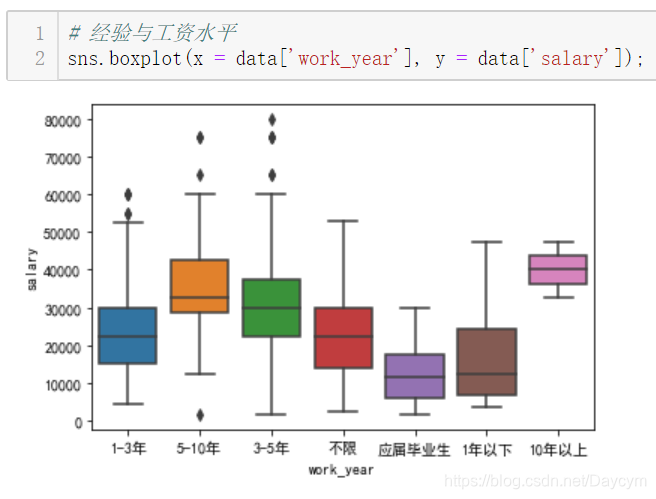
工作年限越长，工资水平越高

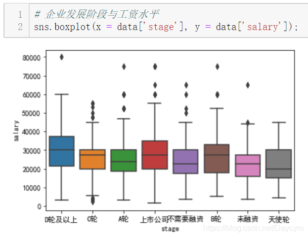
图中，上市公司与D轮及以上稍微高点，B轮的也不低，其实说明有些时候公司在发展中时如果资金允许更愿意多花点钱招入人才

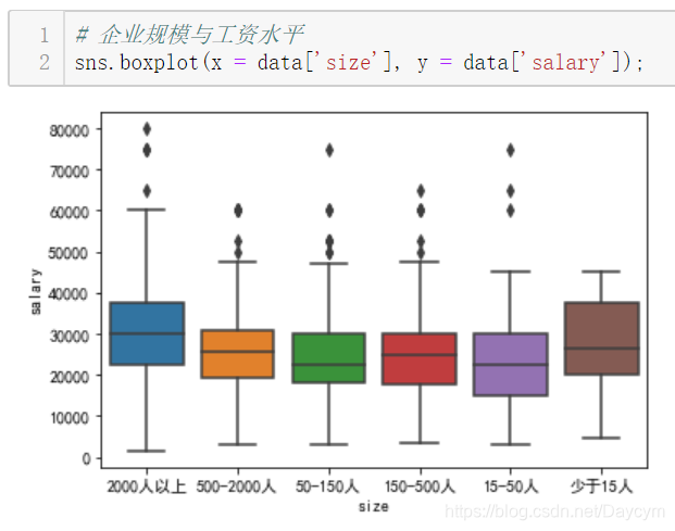
其中，2000人以上的比较高，少于15人的也比较高，可能因为人少的公司一个人要当几个人用，所以工资会给的高点

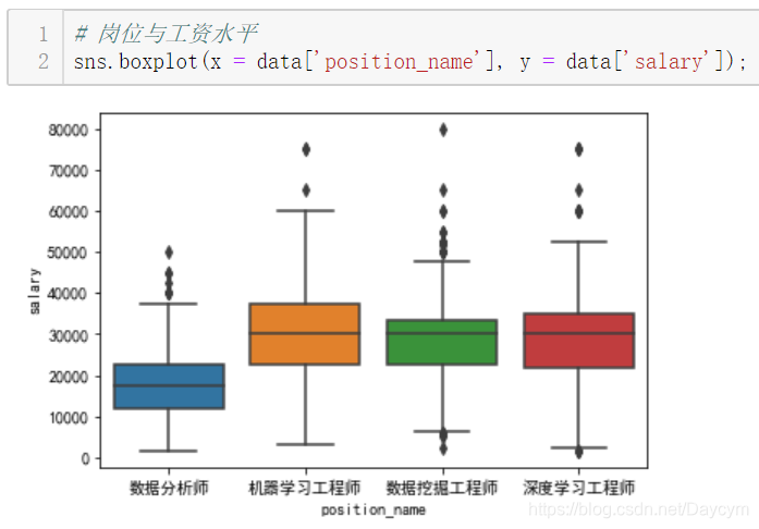
机器学习、数据挖掘、深度学习差不多

# 处理industry变量
for i, j in enumerate(data['industry']):
    if ',' not in j:
        data['industry'][i] = j
    else:
        data['industry'][i] = j.split(',')[0]
        
#data['industry'].value_counts()

industries = ['移动互联网', '金融', '数据服务', '电子商务', '企业服务', '医疗健康', 'O2O', '硬件', '信息安全', '教育']
for i, j in enumerate(data['industry']):
    if j not in industries:
        data['industry'][i] = '其他'
    
#data['industry'].value_counts()

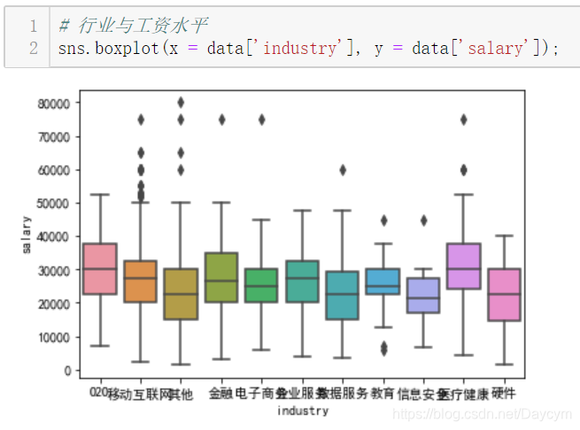
O2O、医疗健康的工资水平较高

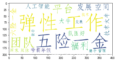
【岗位待遇特征处理：】

• 因为这是个长文本，这里采用了分词，取关键词，画词云图

ADV = []
for i in data['advantage']:
    ADV.append(i)
    
ADV_text = ''.join(ADV)


import jieba
result = jieba.cut(ADV_text)
print("切分结果:  "+",".join(result))

jieba.suggest_freq(('五险一金'), True)
jieba.suggest_freq(('六险一金'), True)
jieba.suggest_freq(('带薪年假'), True)
jieba.suggest_freq(('年度旅游'), True)
jieba.suggest_freq(('氛围好'), True)
jieba.suggest_freq(('技术大牛'), True)
jieba.suggest_freq(('免费三餐'), True)
jieba.suggest_freq(('租房补贴'), True)
jieba.suggest_freq(('大数据'), True)
jieba.suggest_freq(('精英团队'), True)
jieba.suggest_freq(('晋升空间大'), True)

result = jieba.cut(ADV_text)
print("切分结果:  "+",".join(result))

#读取标点符号库
f = open("./stopwords.txt", "r")
stopwords={}.fromkeys(f.read().split("\n"))
f.close()
#加载用户自定义词典
# jieba.load_userdict("./utils/jieba_user_dict.txt")
segs = jieba.cut(ADV_text)
mytext_list=[]
#文本清洗
for seg in segs:
    if seg not in stopwords and seg != " " and len(seg) != 1:
        mytext_list.append(seg.replace(" ", ""))
        
ADV_cloud_text = ",".join(mytext_list)

from wordcloud import WordCloud
wc = WordCloud(
    background_color="white", #背景颜色
    max_words=800, #显示最大词数
    font_path = r'C:\Windows\Fonts\STFANGSO.ttf',  
    min_font_size=15,
    max_font_size=80
    )
wc.generate(ADV_cloud_text)
wc.to_file("ADV_cloud.png")
plt.imshow(wc)
plt.show()

# 剔除几个无用变量
data2 = data.drop(['address', 'industryLables', 'company_name'], axis=1)
data2.shape  # (1650, 11)

五、特征工程

1、特征工程概述

  什么是特征工程？特征工程指的是最大程度上从原始数据中汲取特征和信息来使得模型和算法达到尽可能好的效果。

【特征工程具体内容包括：】

• 数据预处理
• 特征选择
• 特征变换与提取
• 特征组合
• 数据降维

【特征工程的两个基本面：】

• 基于数理和模型的考虑
• 基于业务的考虑（需要了解数据所属业务领域的专业知识）

【几个重要观点：】

• 在实际的特征工程实践中，这两个基本面都要考虑，尤其是业务层面，直接关乎到模型的表现。
• 在数据维度特别大、特征数量极多的情况下，找到数据中的 magic feature 至关重要。
• 总之，数据和特征决定了机器学习效果的上限，模型和算法只是不断地逼近这个上限而已。
• kaggle、天池等数据科学竞赛比模型吗？比算法吗？通通不是，比的是特征工程。

2、数据预处理

• 一些前期的数据清洗和预处理工作，是对原始数据的基本整理和重塑

3、特征选择

  特征选择即选择与目标变量相关的自变量进行用于建模，也叫变量筛选。

【特征选择基于两个基本面：】

• 特征是否发散，即该特征对于模型是否有解释力，如果特征是一成不变的（0方差），这样的特征是无用的。
• 特征是否与目标变量有一定的相关性。这一点要充分基于业务层面去考虑。

【特征选择柳叶三刀：】

• Filter (飞刀)：特征过滤
• Wrapper (弯刀)：特征包装
• Embedded (电刀)：特征嵌入

除了基于pandas和numpy的手动特征选择外，sklearn也有一套特征选择模块。

# 过滤法之方差筛选
from sklearn.feature_selection import VarianceThreshold
X = [[0, 0, 1], [0, 1, 0], [1, 0, 0], [0, 1, 1], [0, 1, 0], [0, 1, 1]]
sel = VarianceThreshold(threshold=(.8 * (1 - .8)))
sel.fit_transform(X)

第一列值为0的比例超过了80%，在结果中VarianceThreshold剔除这一列

# 过滤法之卡方检验
from sklearn.datasets import load_iris
from sklearn.feature_selection import SelectKBest
from sklearn.feature_selection import chi2
iris = load_iris()
X, y = iris.data, iris.target
X.shape
X_new = SelectKBest(chi2, k=2).fit_transform(X, y)
X_new.shape

通过卡方检验筛选2个最好的特征

# 包装法
# 选定一些算法，根据算法在数据上的表现来选择特征集合，一般选用的算法包括随机森林、支持向量机和k近邻等常用算法。
import matplotlib.pyplot as plt
from sklearn.svm import SVC
from sklearn.model_selection import StratifiedKFold
from sklearn.feature_selection import RFECV
from sklearn.datasets import make_classification

X, y = make_classification(n_samples=1000, n_features=25, n_informative=3,n_redundant=2, 
                           n_repeated=0, n_classes=8, n_clusters_per_class=1, random_state=0)

svc = SVC(kernel="linear")
rfecv = RFECV(estimator=svc, step=1, cv=StratifiedKFold(2), scoring='accuracy')
rfecv.fit(X, y)

print("Optimal number of features : %d" % rfecv.n_features_)

plt.figure()
plt.xlabel("Number of features selected")
plt.ylabel("Cross validation score (nb of correct classifications)")
plt.plot(range(1, len(rfecv.grid_scores_) + 1), rfecv.grid_scores_)
plt.show();

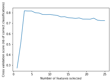
可以发现特征数量在3的时候达到最高

# 嵌入法之基于惩罚项的特征选择法 
from sklearn.svm import LinearSVC
from sklearn.datasets import load_iris
from sklearn.feature_selection import SelectFromModel
iris = load_iris()
X, y = iris.data, iris.target
print('原始数据特征维度：', X.shape)
lsvc = LinearSVC(C=0.01, penalty="l1", dual=False).fit(X, y)
model = SelectFromModel(lsvc, prefit=True)
X_new = model.transform(X)
print('l1惩罚处理之后的数据维度：', X_new.shape)

原始数据特征维度： (150, 4)
l1惩罚处理之后的数据维度： (150, 3)

# 嵌入法之基于树模型的特征选择法
from sklearn.ensemble import ExtraTreesClassifier
from sklearn.datasets import load_iris
from sklearn.feature_selection import SelectFromModel
iris = load_iris()
X, y = iris.data, iris.target
print('原始数据特征维度：', X.shape)
clf = ExtraTreesClassifier()
clf = clf.fit(X, y)
clf.feature_importances_  
model = SelectFromModel(clf, prefit=True)
X_new = model.transform(X)
print('l1惩罚处理之后的数据维度：', X_new.shape)

原始数据特征维度： (150, 4)
l1惩罚处理之后的数据维度： (150, 2)

4、特征变换与特征提取

【数据特征逐个处理：】

• 数据标准化：基于列
• 数据区间缩放
• 数据归一化：基于行
• 数值目标变量对数化处理（有必要的情况下）
• 定量特征二值化（有必要的情况下）
• 定性特征哑编码（one-hot）
• 大文本信息提取（效果类似于one-hot）

# one-hot的两种方法
# sklearn onehotencoder
from sklearn.preprocessing import OneHotEncoder
from sklearn.datasets import load_iris
iris = load_iris()
OneHotEncoder().fit_transform(iris.target.reshape((-1,1))).toarray()


# pandas dummies 方法
import pandas as pd
pd.get_dummies(iris.target)

5、特征组合

  在单特征不能取得进一步效果的情况下可尝试不同特征之间的特征组合。特别需要基于业务考量，而不是随意组合。

6、降维

适用于高维数据，成千上万的特征数量，但一般特征情况下不建议使用。

• PCA
• SVD
• LDA
• t-SNE

7、实例：招聘数据的特征工程探索

import warnings
warnings.filterwarnings('ignore')
import numpy as np
import pandas as pd

lagou_df = pd.read_csv('./lagou_data5.csv', encoding='gbk')

# advantage和label这两个特征作用不大，可在最后剔除
# 分类变量one-hot处理
# pandas one-hot方法
pd.get_dummies(lagou_df['city']).head()


# sklearn onehot方法
# 先要硬编码labelcoder
from sklearn.preprocessing import OneHotEncoder
from sklearn.preprocessing import LabelEncoder
lbl = LabelEncoder()
lbl.fit(list(lagou_df['city'].values))
lagou_df['city'] = lbl.transform(list(lagou_df['city'].values))
# 查看硬编码结果
#lagou_df['city'].head()
# 再由硬编码转为one-hot编码
df_city = OneHotEncoder().fit_transform(lagou_df['city'].values.reshape((-1,1))).toarray()
#df_city[:5]


# 分类特征统一one-hot处理
cat_features = ['city', 'industry', 'education', 'position_name', 'size', 'stage', 'work_year']
for col in cat_features:
    temp = pd.get_dummies(lagou_df[col])
    lagou_df = pd.concat([lagou_df, temp],axis=1)
    lagou_df = lagou_df.drop([col], axis=1)
    
#lagou_df.shape


pd.options.display.max_columns = 999
lagou_df = lagou_df.drop(['advantage', 'label'], axis=1)
# lagou_df.head()

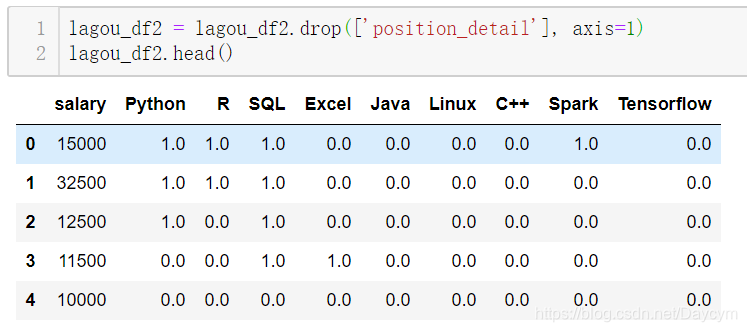
8、职位描述特征的信息提取

lagou_df2 = pd.read_csv('./lagou_data5.csv', encoding='gbk')
lagou_df2 = lagou_df2[['position_detail', 'salary']]

# 提取Python信息
for i, j in enumerate(lagou_df2['position_detail']):
    if 'python' in j:
        lagou_df2['position_detail'][i] = j.replace('python', 'Python')


lagou_df2['Python'] = pd.Series()
for i, j in enumerate(lagou_df2['position_detail']):
    if 'Python' in j:
        lagou_df2['Python'][i] = 1
    else:
        lagou_df2['Python'][i] = 0
        
lagou_df2['Python'][:20]

# 提取R信息
lagou_df2['R'] = pd.Series()
for i, j in enumerate(lagou_df2['position_detail']):
    if 'R' in j:
        lagou_df2['R'][i] = 1
    else:
        lagou_df2['R'][i] = 0
        
lagou_df2['R'].value_counts()


# 提取SQL信息
for i, j in enumerate(lagou_df2['position_detail']):
    if 'sql' in j:
        lagou_df2['position_detail'][i] = j.replace('sql', 'SQL')

lagou_df2['SQL'] = pd.Series()
for i, j in enumerate(lagou_df2['position_detail']):
    if 'SQL' in j:
        lagou_df2['SQL'][i] = 1
    else:
        lagou_df2['SQL'][i] = 0
        
lagou_df2['SQL'].value_counts()

# 提取Excel信息
lagou_df2['Excel'] = pd.Series()
for i, j in enumerate(lagou_df2['position_detail']):
    if 'Excel' in j:
        lagou_df2['Excel'][i] = 1
    else:
        lagou_df2['Excel'][i] = 0
        
lagou_df2['Excel'].value_counts()

# 提取Java信息
lagou_df2['Java'] = pd.Series()
for i, j in enumerate(lagou_df2['position_detail']):
    if 'Java' in j:
        lagou_df2['Java'][i] = 1
    else:
        lagou_df2['Java'][i] = 0
        
lagou_df2['Java'].value_counts()


# 提取Linux信息
for i, j in enumerate(lagou_df2['position_detail']):
    if 'linux' in j:
        lagou_df2['position_detail'][i] = j.replace('linux', 'Linux')
        
lagou_df2['Linux'] = pd.Series()
for i, j in enumerate(lagou_df2['position_detail']):
    if 'Linux' in j:
        lagou_df2['Linux'][i] = 1
    else:
        lagou_df2['Linux'][i] = 0
        
lagou_df2['Linux'].value_counts()

# 提取C++信息
lagou_df2['C++'] = pd.Series()
for i, j in enumerate(lagou_df2['position_detail']):
    if 'C++' in j:
        lagou_df2['C++'][i] = 1
    else:
        lagou_df2['C++'][i] = 0
        
lagou_df2['C++'].value_counts()


# 提取Spark信息
for i, j in enumerate(lagou_df2['position_detail']):
    if 'spark' in j:
        lagou_df2['position_detail'][i] = j.replace('spark', 'Spark')

lagou_df2['Spark'] = pd.Series()
for i, j in enumerate(lagou_df2['position_detail']):
    if 'Spark' in j:
        lagou_df2['Spark'][i] = 1
    else:
        lagou_df2['Spark'][i] = 0
        
lagou_df2['Spark'].value_counts()

# 提取Tensorflow信息
for i, j in enumerate(lagou_df2['position_detail']):
    if 'tensorflow' in j:
        lagou_df2['position_detail'][i] = j.replace('tensorflow', 'Tensorflow')
        
    if 'TensorFlow' in j:
        lagou_df2['position_detail'][i] = j.replace('TensorFlow', 'Tensorflow')
        
lagou_df2['Tensorflow'] = pd.Series()
for i, j in enumerate(lagou_df2['position_detail']):
    if 'Tensorflow' in j:
        lagou_df2['Tensorflow'][i] = 1
    else:
        lagou_df2['Tensorflow'][i] = 0
        
lagou_df2['Tensorflow'].value_counts()

lagou_df2 = lagou_df2.drop(['position_detail'], axis=1)
lagou_df2.head()

lagou_df = lagou_df.drop(['position_detail', 'salary'], axis=1)

lagou = pd.concat((lagou_df2, lagou_df), axis=1).reset_index(drop=True)
lagou.to_csv('lagou_featured.csv', encoding='gbk')

六、机器学习建模与调优

【模型与算法】

• 模型：一类问题的解题步骤，即一类问题的算法。
• 算法：能够解决特定问题的无歧义、机械、有效的运算流程和规则。

【机器学习中的三要素】

• 模型、策略与算法
• 模型：回归模型、分类模型
• 算法：有了模型和策略之后的优化算法：梯度下降法、牛顿法

【机器学习模型】

• 传统机器学习模型（单模型）
• 集成(ensemble)与提升（boosting）模型
• 神经网络与深度学习

1、sklearn

官网文档：http://sklearn.apachecn.org/cn/0.19.0/

• 预处理
• 降维
• 分类
• 回归
• 聚类
• 模型评估与选择
• …

2、机器学习调参

【机器学习模型的参数有哪些？】

（1）模型训练参数：机器学习需要学习的东西，由训练得出，无需也无法调整

• 神经网络的权重与偏置
• 线性回归的变量系数
• …

（2）模型配置参数

• 优化算法的学习率
• 训练轮数
• 树模型最大深度
• …

（3）机器学习模型参数调整方法

• 手动根据经验和尝试调整
• 网格搜索（Grid Search)
• 贝叶斯调参

3、GBDT、XGBoost、lightGBM

GBDT：梯度提升决策树，XGBoost和lightGBM也属于广义上的GBDT模型

GBDT属于加性模型，构建很多棵CART（分类回归树）并组合

import numpy as np
import matplotlib.pyplot as plt

from sklearn import ensemble
from sklearn import datasets
from sklearn.utils import shuffle
from sklearn.metrics import mean_squared_error

# #############################################################################
# 导入数据
boston = datasets.load_boston()
X, y = shuffle(boston.data, boston.target, random_state=13)
X = X.astype(np.float32)
offset = int(X.shape[0] * 0.9)
X_train, y_train = X[:offset], y[:offset]
X_test, y_test = X[offset:], y[offset:]

# #############################################################################
# 拟合模型
params = {'n_estimators': 500, 'max_depth': 4, 'min_samples_split': 2,
          'learning_rate': 0.01, 'loss': 'ls'}
clf = ensemble.GradientBoostingRegressor(**params)

clf.fit(X_train, y_train)
mse = mean_squared_error(y_test, clf.predict(X_test))
print("MSE: %.4f" % mse)

# #############################################################################
# 绘制训练误差图

# 计算测试误差
test_score = np.zeros((params['n_estimators'],), dtype=np.float64)

for i, y_pred in enumerate(clf.staged_predict(X_test)):
    test_score[i] = clf.loss_(y_test, y_pred)

plt.figure(figsize=(12, 6))
plt.subplot(1, 2, 1)
plt.title('Deviance')
plt.plot(np.arange(params['n_estimators']) + 1, clf.train_score_, 'b-',
         label='Training Set Deviance')
plt.plot(np.arange(params['n_estimators']) + 1, test_score, 'r-',
         label='Test Set Deviance')
plt.legend(loc='upper right')
plt.xlabel('Boosting Iterations')
plt.ylabel('Deviance')

# #############################################################################
# 绘制特征重要性图
feature_importance = clf.feature_importances_
feature_importance = 100.0 * (feature_importance / feature_importance.max())
sorted_idx = np.argsort(feature_importance)
pos = np.arange(sorted_idx.shape[0]) + .5
plt.subplot(1, 2, 2)
plt.barh(pos, feature_importance[sorted_idx], align='center')
plt.yticks(pos, boston.feature_names[sorted_idx])
plt.xlabel('Relative Importance')
plt.title('Variable Importance')
plt.show();

【XGBoost】

### XGBoost
import xgboost as xgb

data = np.random.rand(100000, 10) 
label = np.random.randint(2, size=100000) 
dtrain = xgb.DMatrix(data, label=label, missing = -999.0)

data2 = np.random.rand(5000, 10)
label2 = np.random.randint(2, size=5000)
dtest = xgb.DMatrix(data2, label=label2, missing = -999.0)

params = {'bst:max_depth':2, 'bst:eta':1, 'silent':1, 'objective':'binary:logistic' }
params['nthread'] = 4
params['eval_metric'] = 'auc'

evallist  = [(dtrain,'train'), (dtest,'eval')]

num_round = 50
bst = xgb.train(params, dtrain, num_round, evallist)

bst = xgb.train(params, dtrain, num_round, evallist, early_stopping_rounds=10)

【lightGBM】

### lightGBM
import lightgbm as lgb

data = np.random.rand(100000, 10)
label = np.random.randint(2, size=100000)
train_data = lgb.Dataset(data, label=label)

data2 = np.random.rand(5000, 10)
label2 = np.random.randint(2, size=5000)
test_data = lgb.Dataset(data2, label=label2)

param = {'num_leaves':31, 'num_trees':100, 'objective':'binary', 'metrics': 'binary_error'}
num_round = 10
bst = lgb.train(param, train_data, num_round, valid_sets=[test_data])

num_round = 10
param = {'num_leaves':50, 'num_trees':100, 'objective':'binary'}
lgb.cv(param, train_data, num_round, nfold=5)

bst = lgb.train(param, train_data, 20, valid_sets=test_data, early_stopping_rounds=10)
print(bst.best_iteration)

4、招聘数据的建模：GBDT

import pandas as pd
import numpy as np

df = pd.read_csv('./lagou_featured.csv', encoding='gbk')

pd.options.display.max_columns = 999

import matplotlib.pyplot as plt
plt.hist(df['salary'])

X = df.drop(['salary'], axis=1).values
y = df['salary'].values.reshape((-1, 1))
print(X.shape, y.shape)

from sklearn.model_selection import train_test_split
X_train, X_test, y_train, y_test = train_test_split(X, y, test_size=0.3, random_state=42)
print(X_train.shape, y_train.shape, X_test.shape, y_test.shape)

from sklearn.ensemble import GradientBoostingRegressor
model = GradientBoostingRegressor(n_estimators = 100, max_depth = 5)
model.fit(X_train, y_train)

from sklearn.metrics import mean_squared_error
y_pred = model.predict(X_test)
print(np.sqrt(mean_squared_error(y_test, y_pred)))

plt.plot(y_pred)
plt.plot(y_test)
plt.legend(['y_pred', 'y_test'])
plt.show();

# 目标变量对数化处理
X_train, X_test, y_train, y_test = train_test_split(X, np.log(y), test_size=0.3, random_state=42)
model = GradientBoostingRegressor(n_estimators = 100, max_depth = 5)
model.fit(X_train, y_train)
y_pred = model.predict(X_test)
print(np.sqrt(mean_squared_error(y_test, y_pred)))

plt.plot(np.exp(y_pred))
plt.plot(np.exp(y_test))
plt.legend(['y_pred', 'y_test'])
plt.show();

5、招聘数据建模：XGBoost

from sklearn.model_selection import KFold
import xgboost as xgb
from sklearn.metrics import mean_squared_error
import time


kf = KFold(n_splits=5, random_state=123, shuffle=True)

def evalerror(preds, dtrain):
    labels = dtrain.get_label()
    return 'mse', mean_squared_error(np.exp(preds), np.exp(labels))


y = np.log(y)
valid_preds = np.zeros((330, 5))

time_start = time.time()


for i, (train_ind, valid_ind) in enumerate(kf.split(X)):
    print('Fold', i+1, 'out of', 5)
    X_train, y_train = X[train_ind], y[train_ind]
    X_valid, y_valid = X[valid_ind], y[valid_ind]
    xgb_params = {
        'eta': 0.01, 
        'max_depth': 6, 
        'subsample': 0.9, 
        'colsample_bytree': 0.9, 
        'objective': 'reg:linear', 
        'eval_metric': 'rmse', 
        'seed': 99, 
        'silent': True
    }

    d_train = xgb.DMatrix(X_train, y_train)
    d_valid = xgb.DMatrix(X_valid, y_valid)
    
    watchlist = [(d_train, 'train'), (d_valid, 'valid')]
    model = xgb.train(
        xgb_params, 
        d_train, 
        2000,
        watchlist,
        verbose_eval=100,
#         feval=evalerror,
        early_stopping_rounds=1000
    )
#     valid_preds[:, i] = np.exp(model.predict(d_valid))

# valid_pred = valid_preds.means(axis=1)
# print('outline score：{}'.format(np.sqrt(mean_squared_error(y_pred, valid_pred)*0.5)))
print('cv training time {} seconds'.format(time.time() - time_start))

---

import xgboost as xgb
xg_train = xgb.DMatrix(X, y)

params = {
        'eta': 0.01, 
        'max_depth': 6, 
        'subsample': 0.9, 
        'colsample_bytree': 0.9, 
        'objective': 'reg:linear', 
        'eval_metric': 'rmse', 
        'seed': 99, 
        'silent': True
    }
cv = xgb.cv(params, xg_train, 1000, nfold=5, early_stopping_rounds=800, verbose_eval=100)

6、招聘数据建模：lightGBM

X = df.drop(['salary'], axis=1).values
y = np.log(df['salary'].values.reshape((-1, 1))).ravel()
print(type(X), type(y))

import lightgbm as lgb
from sklearn.model_selection import KFold
from sklearn.metrics import mean_squared_error

def evalerror(preds, dtrain):
    labels = dtrain.get_label()
    return 'mse', mean_squared_error(np.exp(preds), np.exp(labels))

params = {
    'learning_rate': 0.01,
    'boosting_type': 'gbdt',
    'objective': 'regression',
    'metric': 'mse',
    'sub_feature': 0.7,
    'num_leaves': 17,
    'colsample_bytree': 0.7,
    'feature_fraction': 0.7,
    'min_data': 100,
    'min_hessian': 1,
    'verbose': -1,
}

print('begin cv 5-fold training...')
scores = []
start_time = time.time()

kf = KFold(n_splits=5, shuffle=True, random_state=27)
for i, (train_index, valid_index) in enumerate(kf.split(X)):
    print('Fold', i+1, 'out of', 5)
    X_train, y_train = X[train_index], y[train_index]
    X_valid, y_valid = X[valid_index], y[valid_index]
    lgb_train = lgb.Dataset(X_train, y_train)
    lgb_valid = lgb.Dataset(X_valid, y_valid)
    model = lgb.train(params,
                lgb_train,
                num_boost_round=2000,
                valid_sets=lgb_valid,
                verbose_eval=200,
#                feval=evalerror,
               early_stopping_rounds=1000)
#     feat_importance = pd.Series(model.feature_importance(), index=X.columns).sort_values(ascending=False)
#     test_preds[:, i] = model.predict(lgb_valid)
# print('outline score：{}'.format(np.sqrt(mean_squared_error(y_pred, valid_pred)*0.5)))
print('cv training time {} seconds'.format(time.time() - time_start))

八、模型结果展示与报告输出

机器学习数据操作流程文档写作顺序（文字描述+代码）

• 数据采集（可选）
• 数据读入
• 数据清洗
• EDA与可视化（推荐jupyter notebook）
• 特征工程
• 建模过程
• 调优过程（特征工程/机器学习建模/调参/优化）
• 结果输出

1、机器学习分析报告写作方法

  分析报告不是技术实现过程，需要从业务角度根据数据分析结果来给出结论参考；分析报告一定要是文字报告加图表配套；要清楚分析报告的受众，一般是给领导看；不能出现太多的数理和技术字眼。

注意格式：文字和图表

2、一份完整的数据分析/机器学习分析报告通常包括：

【背景介绍】

• 业务背景介绍
• 需求分析
• 目标
• …

【数据来源和数据说明】

• 数据采集描述
• 数据基本状况说明
• 预处理简要描述
• …

【探索性数据分析与数据可视化】

• 描述性数据分析
• 目标变量重点探索
• 各种绘图与数据可视化参考
• 特征工程相关
• …

【机器学习模型部分】

• 模型尝试和实验过程描述
• 模型诊断与调优
• 模型结果展示
• …

【结论与建议】

• 根据模型结果给出结论
• 模型不足之处
• 后续的研究工作
• …

3、实例：数据相关岗位薪资水平影响因素研究分析报告（简要框架）

【背景介绍】

• 大数据、人工智能兴起，企业和高校对数据科学人才需求加大
• 从政府、高校学界、公司业界以及个人等几个方面写
• 最好能找一些人才需求的数据图表、历年各专业毕业生薪资对比

【数据来源和数据说明】

• 从哪采集的数据（不讲采集技术）
• 样本量整体描述

【探索性数据分析与数据可视化】

• 不再是此前在jupter里面的无目标的探索，要根据此前探索的结果进行方向性整合
• 可视化图表需要简单、有效、美观
• 直接展示特征工程的结果，用了哪些特征，创建了哪些新特征，丢弃了哪些特征等等，而不是处理过程

【机器学习模型部分】

• 直接展示最后用了哪一个模型，或者是融合了哪些模型
• 模型诊断调优不需要写太细
• 给出特征重要性，解读模型结果，比如说影响数据科学岗位薪资水平的众多因素中，学历和经验影响最大，会Python/R等编程语言的岗位要比不会的薪资高出许多等等

【结论与建议】

• 根据模型结果给出结论
• 模型不足之处与深度可挖掘的部分

九、总结

以上便是整个机器学习项目的大体全流程，实际项目中绝大部分时间花费在数据的清洗和特征工程上。需要考虑的如下：

• 数据的来源，是已有还是需要爬取或者购买，数据是否平衡（正负样本比例）
• 对于已有数据，我们需要考虑自己的软硬件设备是否满足需求，例如：如果是图像数据并且数据量较大，单个笔记本是无法完成的，自然这个项目也就没法实现；
• 数据清洗与特征工程：缺失值如何处理、长字符串如何处理、如何将描述性特征转为数值型、分类特征如何处理、特征相关性、特征选择等等
• 业务理解，我觉得非常重要，因为自身不了解业务，就无法在数据探索性分析的时候总结出合理的结论便于后面的工作；
• 知识背景，最起码知道不同算法对不同数据的效果，以及适用于怎样的数据，优点，缺点这些，理论知识也知道的话在调参的时候会明白参数的意义在哪里；
• Coding，代码能力当然是不可少的咯，以及相关库的使用，建模能力

【本篇代码及数据：】

• Github链接

【学习路线：】

• 数学方面
  • 三大数学基础课：微积分（极限会求、导数和梯度会求、积分会算）、线性代数（矩阵理论和运算）和概率统计（熟悉随机变量、概率、条件概率、常见分布）
  • 统计学方面（数理统计）：参数估计和假设检验
  • 优化方面：凸优化、随机过程等
• 编程语言
  • Python
  • 编程语言都是相同的，关键在于逻辑和思维
  • 建议：多动手写代码，不要以为看得懂就OK
• 机器学习理论学习
  • 《统计学习方法》李航：理论公式推导，非常强大的一本书
  • 《机器学习》西瓜书，周志华：机器学习全貌，好比地图
  • 《机器学习实战》Peter Harrington：机器学习算法的实现，使用Numpy，帮助理解算法原理
  • 《深度学习》花书：深度学习部分的理论知识
• 实战方面：
  • github上的一些项目
  • 竞赛的项目：kaggle、天池等