机器学习实战-CSDN博客

本文链接：https://blog.csdn.net/Der_ek__/article/details/147288443

基础知识

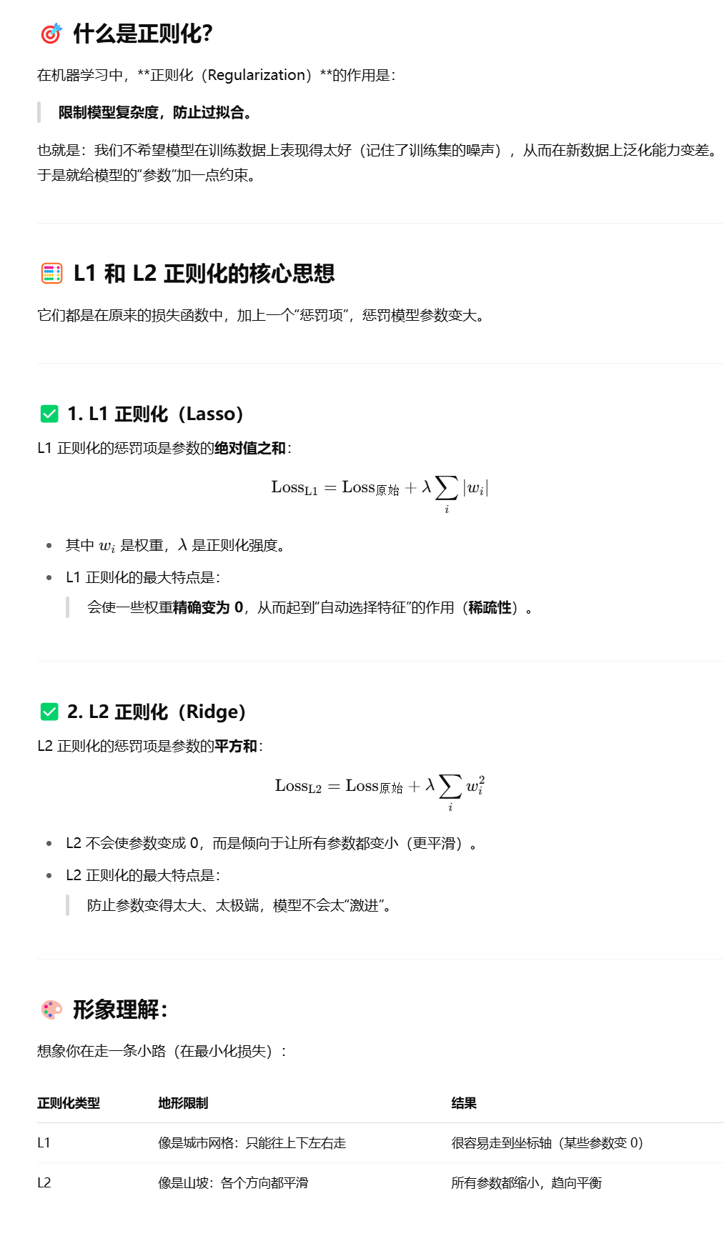
防止过拟合通常1增加数据集2正则化（比较温和）3.降维（把一些冗余特征删除）

线性回归

函数	说明
`np.zeros((3, 4))`	创建 3x4 的零矩阵
`np.ones((2, 2))`	创建 2x2 的全1矩阵
`np.eye(3)`	创建 3x3 的单位矩阵
`np.arange(0, 10, 2)`	[0, 2, 4, 6, 8] 类似 `range`
`np.linspace(0, 1, 5)`	线性等分：[0. , 0.25, 0.5 , 0.75, 1.]

总代码：

import numpy as np
import matplotlib.pyplot as plt

# 数据：面积（x1）、房间数（x2）、房价（y）
X = np.array([
    [50, 2],
    [60, 3],
    [80, 3],
    [100, 4],
    [120, 4],
    [140, 5],
    [160, 5],
    [180, 6],
    [200, 6],
    [220, 7]
], dtype=np.float64)#精度64位浮点数

y = np.array([120, 150, 180, 210, 250, 280, 310, 340, 370, 400], dtype=np.float64)

# 特征归一化（提升收敛速度），提升梯度下降速度
X_mean = np.mean(X, axis=0)
X_std = np.std(X, axis=0)
X = (X - X_mean) / X_std

# 添加一列全为1的偏置项（即x0 = 1）
X = np.hstack((np.ones((X.shape[0], 1)), X))  # X.shape = (10, 3)
'''创建X.shape[0]行1列的全一矩阵#np.ones((X.shape[0], 1))
np.hstack((..., X))hstack 表示“水平拼接”，沿着列的方向，把两个矩阵拼在一起：
左边是全 1 的列（偏置）；右边是原始特征 X。
'''


# 初始化参数 theta（包括 bias）
theta = np.zeros(X.shape[1])  # theta.shape = (3,)

# 设置学习率和迭代次数
alpha = 0.1
epochs = 1000
losses = []

# 梯度下降
for epoch in range(epochs):
    y_pred = X @ theta               # 预测值（矩阵乘法）
    error = y_pred - y               # 预测误差
    loss = (1 / (2 * len(y))) * np.sum(error ** 2)
    losses.append(loss)

    grad = (1 / len(y)) * (X.T @ error)  # 梯度计算
    theta -= alpha * grad               # 参数更新

    if epoch % 100 == 0:
        print(f"Epoch {epoch}, Loss: {loss:.4f}")

print("\n训练完成后的参数：", theta)

# 画出损失下降过程
plt.plot(losses)
plt.title("Loss Curve")
plt.xlabel("Epochs")
plt.ylabel("Loss")
plt.grid()
plt.show()

np库的array用法：切片和索引左闭右开，但是冒号表示到最后

a = np.array([[10, 20, 30],
              [40, 50, 60]])

print(a[0, 1])   # 取第一行第二列：20
print(a[1])      # 取第二行：[40 50 60]
print(a[:, 0])   # 所有行的第一列：[10 40]
print(a[0:2, 1:]) # 子矩阵：从前两行取后两列

矩阵乘法

x = np.array([[1, 2], [3, 4]])   # 2x2 矩阵
w = np.array([[2], [1]])         # 2x1 矩阵

# 矩阵乘法用 @ 或 np.dot
y = x @ w
print(y)
# [[ 4]
#  [10]]

shape的用法

import numpy as np

a = np.array([[1, 2, 3],
              [4, 5, 6]])

print(a.shape)      # 输出：(2, 3)
print(type(a.shape))  # <class 'tuple'>

np.mean和np.std求均值和标准差

b = np.array([[1, 2],
              [3, 4]])

print(np.std(b))            # 所有元素的标准差
print(np.std(b, axis=0))    # 每列的标准差
print(np.std(b, axis=1))    # 每行的标准差

标准化举例，（原数据-均值）/标准差

标准化（Z-score Normalization）：
x′=x−μσx′=σx−μ
使数据均值为0，方差为1，适用于大部分深度学习模型（如DNN、CNN）。

学习率固定，如果有的特征相较于其他特征特别大就容易震荡。

import numpy as np

X = np.array([[1, 2],
              [3, 4],
              [5, 6]], dtype=np.float64)

X_mean = np.mean(X, axis=0)  # 每列平均值 → [3. 4.]
X_std = np.std(X, axis=0)    # 每列标准差 → [1.6329 1.6329]

X_standardized = (X - X_mean) / X_std

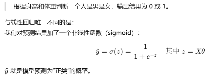
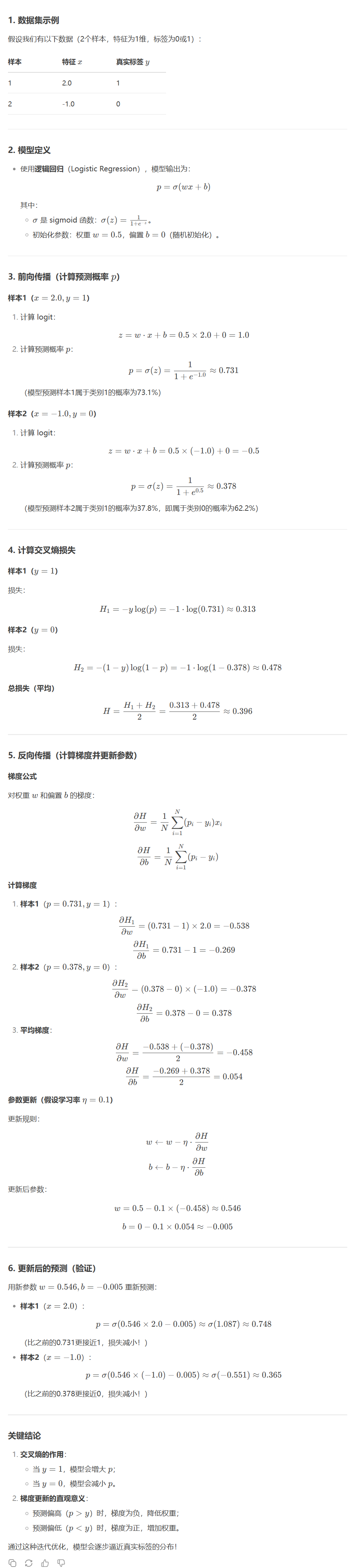
对数几率回归

正负样本，正样本是符合分类预期的，比如垃圾邮件检测中的垃圾邮件。

损失函数是衡量单个样本的，

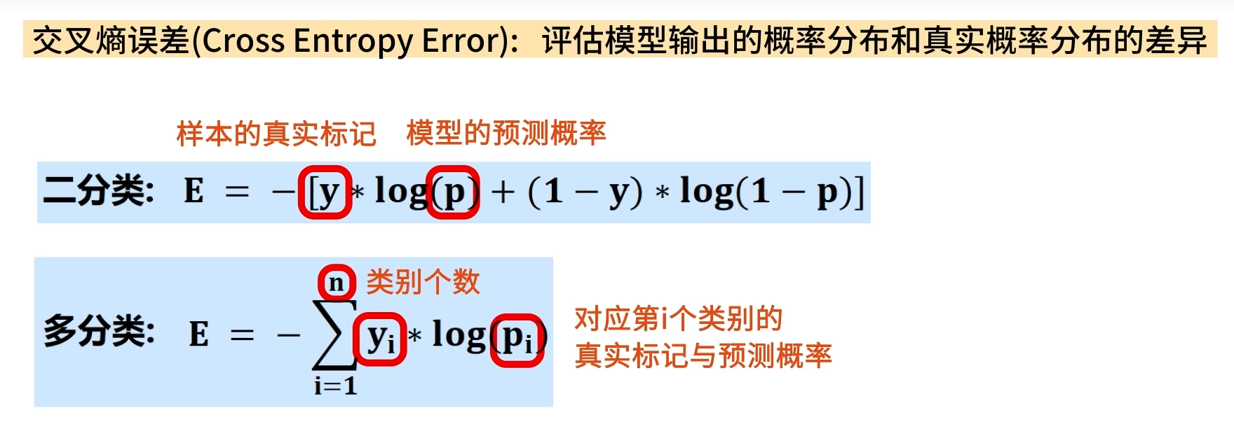
交叉损失熵

import numpy as np

# 模拟数据（两个特征，二分类）
X = np.array([
    [2, 3],
    [1, 5],
    [2, 8],
    [5, 2],
    [6, 1],
    [7, 3]
], dtype=np.float64)

y = np.array([0, 0, 0, 1, 1, 1], dtype=np.float64)

# 数据归一化（可选但推荐）
X_mean = np.mean(X, axis=0)
X_std = np.std(X, axis=0)
X = (X - X_mean) / X_std

# 添加偏置项
X = np.hstack((np.ones((X.shape[0], 1)), X))  # shape: (6, 3)

# Sigmoid 函数
def sigmoid(z):
    return 1 / (1 + np.exp(-z))

# 损失函数（交叉熵）
def compute_loss(y_pred, y_true):
    epsilon = 1e-8  # 避免 log(0)
    return -np.mean(y_true * np.log(y_pred + epsilon) + (1 - y_true) * np.log(1 - y_pred + epsilon))

# 初始化参数
theta = np.zeros(X.shape[1])  # shape: (3,)

# 超参数
lr = 0.1
num_iters = 1000

# 梯度下降训练过程
for i in range(num_iters):
    z = X @ theta                 # 线性部分
    y_pred = sigmoid(z)          # 预测概率
    error = y_pred - y           # 残差
    grad = (1 / len(y)) * (X.T @ error)  # 梯度
    theta -= lr * grad           # 参数更新

    if i % 100 == 0:
        loss = compute_loss(y_pred, y)
        print(f"Iteration {i}, Loss: {loss:.4f}")

# 最终参数
print("Final theta:", theta)

# 预测函数
def predict(x_new):
    x_new = (x_new - X_mean) / X_std           # 特征归一化
    x_new = np.insert(x_new, 0, 1.0)           # 加偏置项
    prob = sigmoid(np.dot(x_new, theta))       # 概率
    return 1 if prob >= 0.5 else 0, prob

# 测试预测
x_test = np.array([4, 3])  # 一个新样本
cls, prob = predict(x_test)
print(f"Test sample {x_test} → Predict: class={cls}, prob={prob:.4f}")

小知识点

layer_1 = Dense(units=3, activation='sigmoid')
layer_1(x)

units=3
表示该层有 3 个神经元，即输出一个 3 维向量（形状为 (batch_size, 3)）。
activation='sigmoid'
表示该层的激活函数是 Sigmoid

假设输入是一个向量 xx（形状为 (batch_size, input_dim)），则该层的计算步骤如下：

线性变换（加权和 + 偏置）：
z=xW+b
- WW 是权重矩阵，形状为 (input_dim, 3)。
- bb 是偏置向量，形状为 (3,)。
非线性激活（Sigmoid）：
a=σ(z)
输出的 aa 是 3 维向量，每个元素在 (0, 1) 之间。

Dense类的代码（简单示意版）

import torch
import torch.nn as nn
import torch.nn.functional as F
import math

class Dense(nn.Module):
    def __init__(self, units, activation=None):
        super(Dense, self).__init__()
        self.units = units
        self.activation = activation
        
        # 权重和偏置会在第一次前向传播时初始化（知道输入维度后）
        self.weight = None
        self.bias = None
        self.input_dim = None

    def forward(self, x):
        # 如果是第一次运行，初始化权重和偏置
        if self.weight is None:
            self.input_dim = x.shape[-1]  # 输入的特征维度
            # 初始化权重 (input_dim, units)
            self.weight = nn.Parameter(
                torch.Tensor(self.input_dim, self.units)
            )
            # 初始化偏置 (units,)
            self.bias = nn.Parameter(torch.Tensor(self.units))
            # 使用 Xavier/Glorot 初始化
            nn.init.xavier_uniform_(self.weight)
            nn.init.zeros_(self.bias)

        # 计算线性变换: x @ W + b
        output = torch.matmul(x, self.weight) + self.bias
        
        # 应用激活函数
        if self.activation == 'sigmoid':
            output = torch.sigmoid(output)
        elif self.activation == 'relu':
            output = F.relu(output)
        # 其他激活函数...
        
        return output

layer_1被实例化为Dense的对象，forword方法被__call__重写，帮助其可以被像函数一样调用。