


一、简介:淡水质量预测
问题描述:
淡水是我们最重要和最稀缺的自然资源之一,仅占地球总水量的 3%。它几乎触及我们日常生活的方方面面,从饮用、游泳和沐浴到生产食物、电力和我们每天使用的产品。获得安全卫生的供水不仅对人类生活至关重要,而且对正在遭受干旱、污染和气温升高影响的周边生态系统的生存也至关重要。
预期解决方案:
通过参考英特尔的类似实现方案,预测淡水是否可以安全饮用和被依赖淡水的生态系统所使用,从而可以帮助全球水安全和环境可持续性发展。这里分类准确度和推理时间将作为评分的主要依据。
数据集:https://filerepo.idzcn.com/hack2023/datasetab75fb3.zip
二、数据探索
查看数据规模和部分数据:
data = pd.read_csv('dataset.csv')
print('数据规模:{}\n'.format(data.shape))
display(data.head())
data=data.infer_objects()
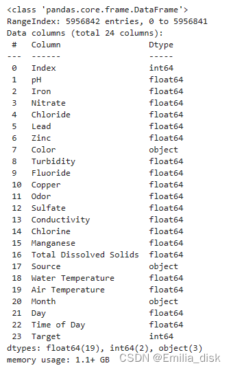
data.info()可以看到数据有5956842行,除开序号有23个类别,其中Color、Source、Month是object数据类型,Index、Target是int64数据类型,其他则是float64数据类型。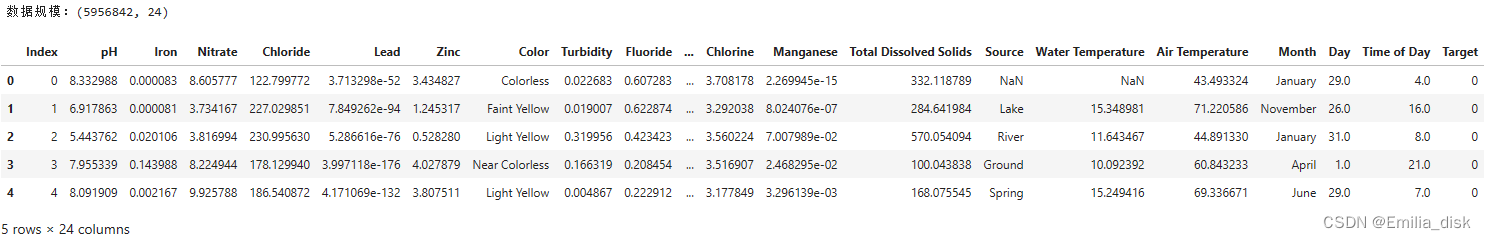
转换数据类型:
Color、Source、Month都是字符串不能直接进行数学统计, 将这三个字段因子化处理成数字变量。
factor = pd.factorize(data['Color'])
print(factor)
data.Color = factor[0]
factor = pd.factorize(data['Source'])
print(factor)
data.Source = factor[0]
factor = pd.factorize(data['Month'])
print(factor)
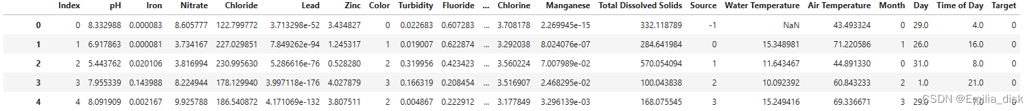
data.Month = factor[0]
data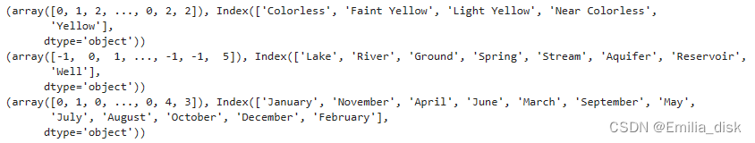
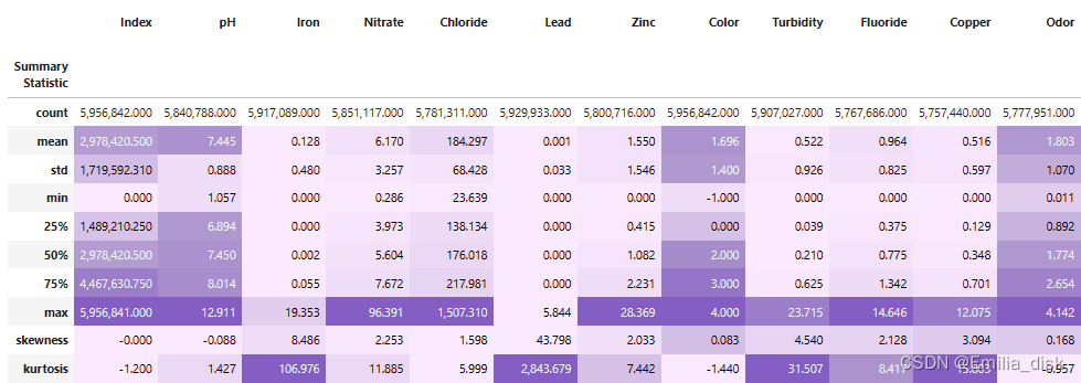
 查看数据特征:
from matplotlib.colors import LinearSegmentedColormap
colors = ['#FBEAFF',"#B39CD0","#845Ec2"]
cmap = LinearSegmentedColormap.from_list("mycmap", colors)
def display_stats(df):

    """
    Function to display descriptive statistics of numerical variables,
    includes skewness & kurtosis.
    """

    df=data.describe()
    skewness=data.skew()
    kurtosis=data.kurtosis()
    df = pd.concat([df, pd.DataFrame([skewness, kurtosis])], ignore_index=True)
    idx=pd.Series(['count','mean','std','min','25%','50%','75%',
                    'max','skewness','kurtosis'],name='Summary Statistic')
    df=pd.concat([df,idx],1).set_index('Summary Statistic')
    display(df.style.format('{:,.3f}').
        background_gradient(subset=(df.index[1:],df.columns[:]),
                            cmap=cmap))

display_stats(data)
通过查看各个字段的统计特征,了解数据的峰度和偏度。
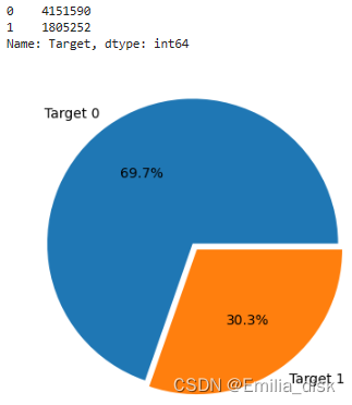
查看标签数量:
print(data.Target.value_counts())
target = data.Target.value_counts()
target.rename(index={1: 'Target 1', 0: 'Target 0'}, inplace=True)
plt.pie(target, [0, 0.05], target.index, autopct='%1.1f%%')
plt.show()
通过饼状图直观了解数据中淡水质量好和坏的数量分布。数据中淡水质量好的接近70%,剩下30%的淡水质量都不够好,数据有些不平衡。
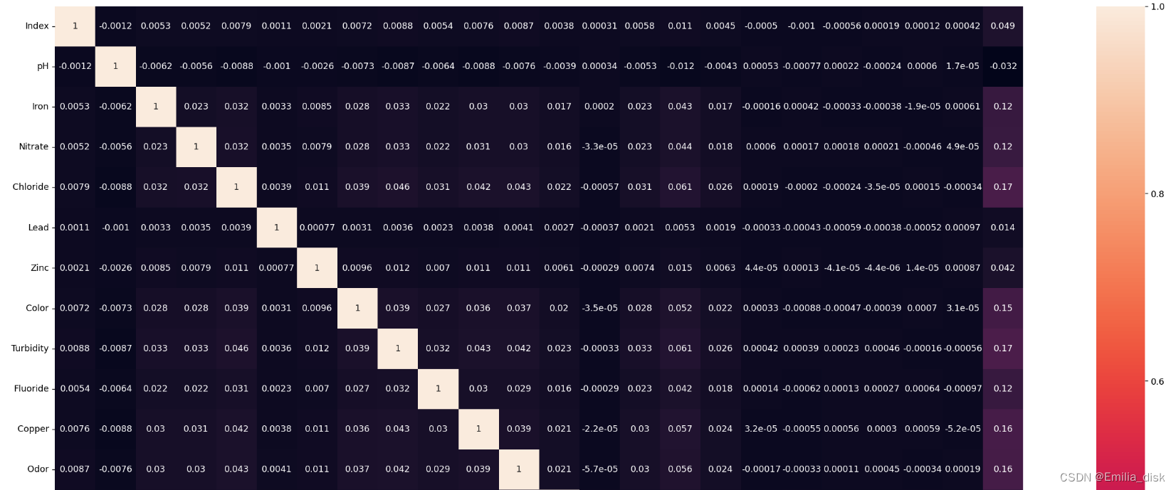
查看数据热力图:
corr = plt.subplots(figsize = (30,20),dpi=128)
corr= sns.heatmap(data.corr(method='spearman'),annot=True,square=True)
这里可以发现各个属性间的相关性并不高。
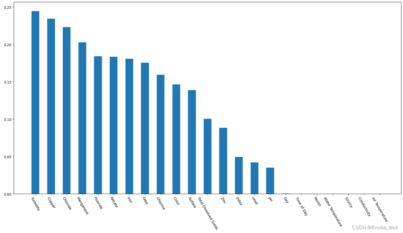
相关性分析:
import matplotlib.pyplot as plt;
import numpy as np
# 相关性分析
bar = data.corr()['Target'].abs().sort_values(ascending=False)[1:]

plt.bar(bar.index, bar, width=0.5)
# 设置figsize的大小
pos_list = np.arange(len(data.columns))
params = {
    'figure.figsize': '20, 10'
}
plt.rcParams.update(params)
plt.xticks(bar.index, bar.index, rotation=-60, fontsize=10)
plt.show()
通过柱状图来查看各个字段对Target的影响程度,观察图像可以发现Day、Time of Day、Water Temperature、Conductivity、Air Temperature、Month、Source和Target间的相关性很低,Index字段的相关性没有价值。
将相关性不高和没有价值的列删去
data =data.drop(
    columns=['Index', 'Day', 'Time of Day', 'Water Temperature',
             'Conductivity', 'Air Temperature','Month','Source'],axis=1)
三、数据预处理
处理数据缺失值和重复值:
查看缺失值和重复值
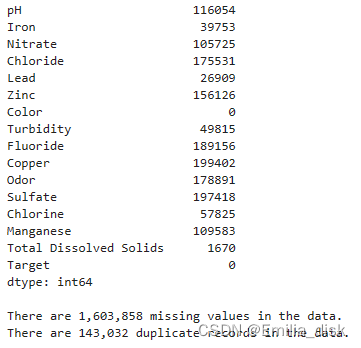
display(data.isna().sum())
missing = data.isna().sum().sum()
duplicates = data.duplicated().sum()
print("\nThere are {:,.0f} missing values in the data.".format(missing))
print("There are {:,.0f} duplicate records in the data.".format(duplicates))
可以看到除Target和Color字段都有许多数据值为空。
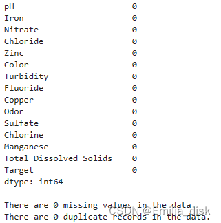
将数据为空的值用0填充,再删除重复的值
data = data.fillna(0)
data = data.drop_duplicates()
偏差值处理:
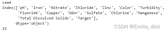
进行偏差值处理,删除数据中偏差较大的值,这里使用了scipy.stats 模块中的 pearsonr 函数,用于计算两个变量之间的皮尔逊相关系数和 p 值。这里先判断每一列的方差是否小于等于 0.1,如果是,则认为该列的变化程度较低,对目标变量的影响较小,不适合作为特征,将被去掉。再计算每一列与目标变量之间的皮尔逊相关系数和 p 值,判断 p 值是否大于 0.05,如果是,则认为该列与目标变量之间的相关性不显著,不适合作为特征。
from scipy.stats import pearsonr

variables = data.columns
df = data

var = df.var()
numeric = df.columns
df = df.fillna(0)
for i in range(0, len(var) - 1):
    if var[i] <= 0.1:  # 方差大于10%
        print(variables[i])
        df = df.drop(numeric[i], axis=1)
variables = df.columns

for i in range(0, len(variables)):
    x = df[variables[i]]
    y = df[variables[-1]]
    if pearsonr(x, y)[1] > 0.05:
        print(variables[i])
        df = df.drop(variables[i], axis=1)

variables = df.columns
print(variables)
print(len(variables))
处理后删除了Lead这一列
再查看数据的缺失值和重复值已经全部处理好了
四、初步模型拟合:
数据划分和图像分析:
下面三个函数分别是数据划分和图像绘制。第一个将数据集按比例划分训练集和测试集,第二个用来绘制AUC和AUPRC的图像,第三个是绘制预测测试集Target分布的饼状图。
import plotly.io as pio
pio.renderers.default = "iframe"
# 定义 intel_pal 为一个列表,包含一些颜色
intel_pal=['#0071C5','#FCBB13']
color=['#7AB5E1','#FCE7B2']
def prepare_train_test_data(data, target_col, test_size):
scaler = RobustScaler()
X = data.drop(target_col, axis=1)
y = data[target_col]
X_train, X_test, y_train, y_test = train_test_split(X, y, test_size=test_size, random_state=21)
X_train_scaled = scaler.fit_transform(X_train)
X_test_scaled = scaler.transform(X_test)
print("Train Shape: {}".format(X_train_scaled.shape))
print("Test Shape: {}".format(X_test_scaled.shape))
return X_train_scaled, X_test_scaled, y_train, y_test
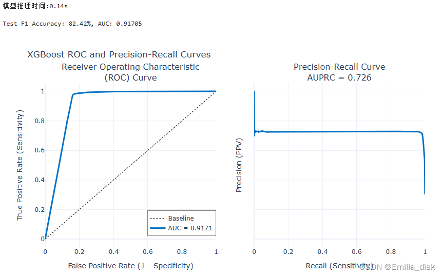
def plot_model_res(model_name, y_test, y_prob):
fpr, tpr, _ = roc_curve(y_test, y_prob)
roc_auc = auc(fpr,tpr)
precision, recall, _ = precision_recall_curve(y_test, y_prob)
auprc = average_precision_score(y_test, y_prob)
fig = make_subplots(rows=1, cols=2,
shared_yaxes=True,
subplot_titles=['Receiver Operating Characteristic<br>(ROC) Curve',
'Precision-Recall Curve<br>AUPRC = {:.3f}'.format(auprc)])
fig.add_trace(go.Scatter(x=np.linspace(0,1,11), y=np.linspace(0,1,11),
name='Baseline',mode='lines',legendgroup=1,
line=dict(color="Black", width=1, dash="dot")), row=1,col=1)
fig.add_trace(go.Scatter(x=fpr, y=tpr, line=dict(color=intel_pal[0], width=3),
hovertemplate = 'True positive rate = %{y:.3f}, False positive rate = %{x:.3f}',
name='AUC = {:.4f}'.format(roc_auc),legendgroup=1), row=1,col=1)
fig.add_trace(go.Scatter(x=recall, y=precision, line=dict(color=intel_pal[0], width=3),
hovertemplate = 'Precision = %{y:.3f}, Recall = %{x:.3f}',
name='AUPRC = {:.4f}'.format(auprc),showlegend=False), row=1,col=2)
fig.update_layout(template='plotly_white', title="{} ROC and Precision-Recall Curves".format(model_name),
hovermode="x unified", width=900,height=500,
xaxis1_title='False Positive Rate (1 - Specificity)',
yaxis1_title='True Positive Rate (Sensitivity)',
xaxis2_title='Recall (Sensitivity)',yaxis2_title='Precision (PPV)',
legend=dict(orientation='v', y=.07, x=.45, xanchor="right",
bordercolor="black", borderwidth=.5))
fig.show()
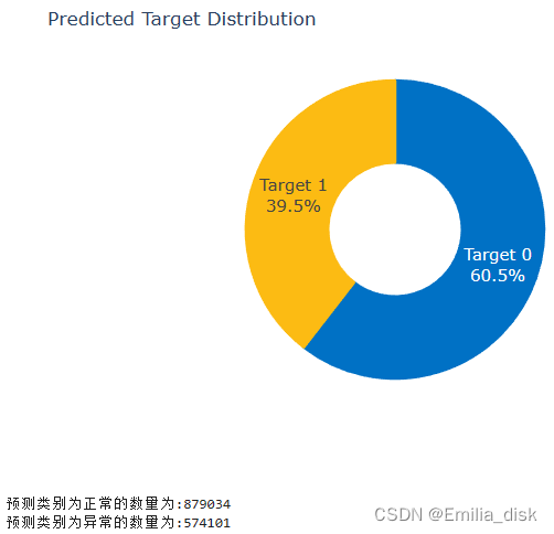
def plot_distribution(y_prob):
plot_df=pd.DataFrame.from_dict({'Target 0':(len(y_prob[y_prob<=0.5])/len(y_prob))*100,
'Target 1':(len(y_prob[y_prob>0.5])/len(y_prob))*100},
orient='index', columns=['pct'])
fig=go.Figure()
fig.add_trace(go.Pie(labels=plot_df.index, values=plot_df.pct, hole=.45,
text=plot_df.index, sort=False, showlegend=False,
marker=dict(colors=intel_pal,line=dict(color=intel_pal,width=2.5)),
hovertemplate = "%{label}: <b>%{value:.2f}%</b><extra></extra>"))
fig.update_layout(template='plotly_white', title='Predicted Target Distribution',width=700,height=450,
uniformtext_minsize=15, uniformtext_mode='hide')
fig.show()用原始数据加XGBClassifier:
from sklearn.preprocessing import RobustScaler
from sklearn.model_selection import train_test_split
from xgboost import XGBClassifier
from sklearn.model_selection import StratifiedKFold
from sklearn.model_selection import GridSearchCV
import time
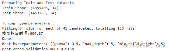
## Prepare Train and Test datasets ##
print("Preparing Train and Test datasets")
X_train, X_test, y_train, y_test = prepare_train_test_data(data=df,
target_col='Target',
test_size=.25)
## Initialize XGBoost model ##
ratio = float(np.sum(y_train == 0)) / np.sum(y_train == 1)
parameters = {'scale_pos_weight': ratio.round(2),
'tree_method': 'hist',
'random_state': 21}
xgb_model = XGBClassifier(**parameters)
## Tune hyperparameters ##
strat_kfold = StratifiedKFold(n_splits=3, shuffle=True, random_state=21)
print("\nTuning hyperparameters..")
grid = {'min_child_weight': [1, 5, 10],
'gamma': [0.5, 1, 1.5, 2, 5],
'max_depth': [3, 4, 5],
}
grid_search = GridSearchCV(xgb_model, param_grid=grid,
cv=strat_kfold, scoring='roc_auc',
verbose=1, n_jobs=-1)
start = time.time()
grid_search.fit(X_train, y_train)
end = time.time()
print('模型拟合时间:{:.2f}'.format(end-start))
print("Done!\nBest hyperparameters:", grid_search.best_params_)
print("Best cross-validation AUC: {:.4f}".format(grid_search.best_score_))
## Convert XGB model to daal4py ##
xgb = grid_search.best_estimator_
#xgb.save_model('xgb_model_raw.model')
daal_model = d4p.get_gbt_model_from_xgboost(xgb.get_booster())
start = time.time()
## Calculate predictions ##
daal_prob = d4p.gbt_classification_prediction(nClasses=2,
resultsToEvaluate="computeClassLabels|computeClassProbabilities",
fptype='float').compute(X_test, daal_model).probabilities # or .predictions
end = time.time()
xgb_pred = pd.Series(np.where(daal_prob[:,1]>.5, 1, 0), name='Target')
xgb_auc = roc_auc_score(y_test, daal_prob[:,1])
xgb_f1 = f1_score(y_test, xgb_pred)
## Plot model results ##
print('模型推理时间:{:.2f}s'.format(end-start))
print("\nTest F1 Accuracy: {:.2f}%, AUC: {:.5f}".format(xgb_f1*100, xgb_auc))
plot_model_res(model_name='XGBoost', y_test=y_test, y_prob=daal_prob[:,1])
plot_distribution(daal_prob[:,1])
print('预测类别为正常的数量为:{:d}'.format(len(daal_prob[:,1][daal_prob[:,1]<=0.5])))
print('预测类别为异常的数量为:{:d}'.format(len(daal_prob[:,1][daal_prob[:,1]>=0.5])))测试集的F1分数为82.42%,准确率为0.91705。
使用课程测试集:
按照之前的步骤处理测试数据。
new_test = pd.read_csv('test_data.csv')
new_test = new_test.drop(columns=['Index', 'Day', 'Time of Day', 'Water Temperature', 'Conductivity', 'Air Temperature','Month','Source','Lead'],axis=1)

factor = pd.factorize(new_test['Color'])
print(factor)
new_test.Color = factor[0]

display(new_test.isna().sum())
missing = new_test.isna().sum().sum()
duplicates = new_test.duplicated().sum()
print("\nThere are {:,.0f} missing values in the data.".format(missing))
print("There are {:,.0f} duplicate records in the data.".format(duplicates))

new_test = new_test.fillna(0)
new_test = new_test.drop_duplicates()
display(new_test.isna().sum())
missing = new_test.isna().sum().sum()
duplicates = new_test.duplicated().sum()
print("\nThere are {:,.0f} missing values in the data.".format(missing))
print("There are {:,.0f} duplicate records in the data.".format(duplicates))
将处理好的数据通过模型来进行预测
X = new_test.drop('Target', axis=1)
y = new_test['Target']
scaler = RobustScaler()
X_test_scaled = scaler.fit_transform(X)
print("Test Shape: {}".format(X_test_scaled.shape))
new_test_scaled = scaler.fit_transform(X_test_scaled)
## Convert XGB model to daal4py ##
xgb = grid_search.best_estimator_
daal_model = d4p.get_gbt_model_from_xgboost(xgb.get_booster())
start = time.time()
## Calculate predictions ##
daal_prob = d4p.gbt_classification_prediction(nClasses=2,
resultsToEvaluate="computeClassLabels|computeClassProbabilities",
fptype='float').compute(new_test_scaled, daal_model).probabilities # or .predictions
end = time.time()
xgb_pred = pd.Series(np.where(daal_prob[:,1]>.5, 1, 0), name='Target')
xgb_auc = roc_auc_score(y, daal_prob[:,1])
xgb_f1 = f1_score(y, xgb_pred)
## Plot model results ##
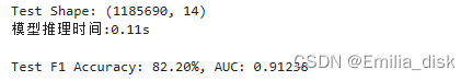
print('模型推理时间:{:.2f}s'.format(end-start))
print("\nTest F1 Accuracy: {:.2f}%, AUC: {:.5f}".format(xgb_f1*100, xgb_auc))课程测试集结果和之前相差不大,F1分数为82.20%,推理时间为0.11s。
五、插值数据进行模型拟合
进行过拟合和欠拟合:
这里使用smote对数据表的特征和目标变量进行过采样,平衡变量Target的数量,让数据更加平衡。这里让Target为0的数据平衡为Target为1数据的一半。
from imblearn.over_sampling import SMOTE
smote_model = SMOTE(k_neighbors=2,random_state=42,sampling_strategy=0.5)
# imblearn 中过采样接口提供了随机过采样 RandomOverSampler、SMOTE、ADASYN 三种方式,调用方式基本一致。
# SMOTE 只适合处理连续性变量特征,不适合离散型特征。
x_smote,y_smote = smote_model.fit_resample(df.iloc[:,:-1],df['Target'])
df_smote = pd.concat([x_smote, y_smote], axis=1)
df_smote.groupby('Target').count()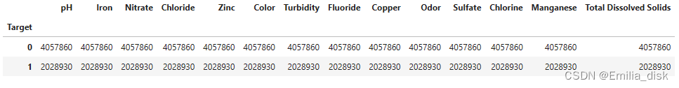
再对数据表进行过采样和欠采样,再多次平衡变量Target的数量。
from imblearn.over_sampling import RandomOverSampler
from imblearn.under_sampling import RandomUnderSampler
rus = RandomUnderSampler(random_state=0,sampling_strategy=0.5)
ros = RandomOverSampler(random_state=0,sampling_strategy=0.5)
X_resampled, y_resampled = ros.fit_resample(df.iloc[:,:-1],df['Target'])
df_resampled = pd.concat([X_resampled, y_resampled], axis=1)
X_uresampled, y_uresampled = rus.fit_resample(df.iloc[:,:-1],df['Target'])
df_uresampled = pd.concat([X_uresampled, y_uresampled], axis=1)
df_new = pd.concat([df_smote, df_resampled[df_resampled['Target']==1.0]], axis=0)
df_new = pd.concat([df_new[df_new['Target']==1.0],df_uresampled[df_uresampled['Target']==0.0]])
df_new.groupby('Target').count()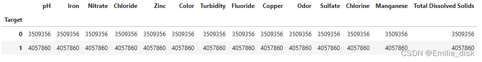
用插值数据进行模型拟合:
## Prepare Train and Test datasets ##
print("Preparing Train and Test datasets")
X_train, X_test, y_train, y_test = prepare_train_test_data(data=df_new,
target_col='Target',
test_size=.25)
## Initialize XGBoost model ##
ratio = float(np.sum(y_train == 0)) / np.sum(y_train == 1)
parameters = {'scale_pos_weight': ratio.round(2),
'tree_method': 'hist',
'random_state': 21}
xgb_model = XGBClassifier(**parameters)
## Tune hyperparameters ##
strat_kfold = StratifiedKFold(n_splits=3, shuffle=True, random_state=21)
print("\nTuning hyperparameters..")
grid = {'min_child_weight': [1, 5, 10],
'gamma': [0.5, 1, 1.5, 2, 5],
'max_depth': [3, 4, 5],
}
grid_search = GridSearchCV(xgb_model, param_grid=grid,
cv=strat_kfold, scoring='roc_auc',
verbose=1, n_jobs=-1)
start = time.time()
grid_search.fit(X_train, y_train)
end = time.time()
print('模型拟合时间:{:.2f}'.format(end-start))
print("Done!\nBest hyperparameters:", grid_search.best_params_)
print("Best cross-validation AUC: {:.4f}".format(grid_search.best_score_))
## Convert XGB model to daal4py ##
xgb = grid_search.best_estimator_
daal_model = d4p.get_gbt_model_from_xgboost(xgb.get_booster())
#xgb.save_model('xgb_model.model')
start = time.time()
## Calculate predictions ##
daal_prob = d4p.gbt_classification_prediction(nClasses=2,
resultsToEvaluate="computeClassLabels|computeClassProbabilities",
fptype='float').compute(X_test, daal_model).probabilities # or .predictions
end = time.time()
xgb_pred = pd.Series(np.where(daal_prob[:,1]>.5, 1, 0), name='Target')
xgb_auc = roc_auc_score(y_test, daal_prob[:,1])
xgb_f1 = f1_score(y_test, xgb_pred)
## Plot model results ##
print('模型推理时间:{:.2f}s'.format(end-start))
print("\nTest F1 Accuracy: {:.2f}%, AUC: {:.5f}".format(xgb_f1*100, xgb_auc))
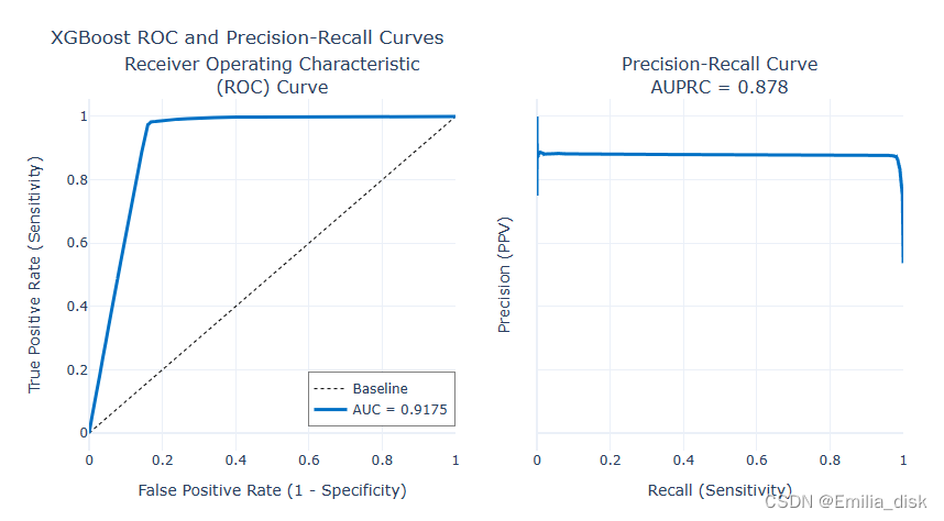
plot_model_res(model_name='XGBoost', y_test=y_test, y_prob=daal_prob[:,1])
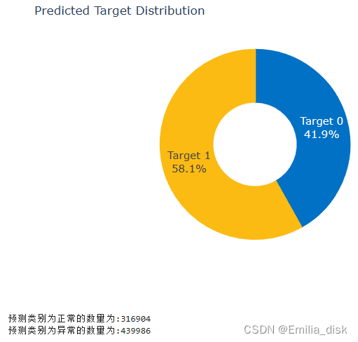
plot_distribution(daal_prob[:,1])
print('预测类别为正常的数量为:{:d}'.format(len(daal_prob[:,1][daal_prob[:,1]<=0.5])))
print('预测类别为异常的数量为:{:d}'.format(len(daal_prob[:,1][daal_prob[:,1]>=0.5])))结果如下,F1分数相较于未插值之前的数据提升了到了91.17%。AUC的提升不大,但是AUCPRC从0.726提成到0.878。


使用课程测试集:
处理测试集后并进行插值处理再导入上面训练的模型进行测试。
X = df_new.drop('Target', axis=1)
y = df_new['Target']
# 创建一个RobustScaler对象,用于对数据进行缩放
scaler = RobustScaler()
# 对特征矩阵进行拟合和转换,得到缩放后的测试集特征X_test_scaled
X_test_scaled = scaler.fit_transform(X)
# 打印出缩放后的测试集特征的形状
print("Test Shape: {}".format(X_test_scaled.shape))
new_test_scaled = scaler.fit_transform(X_test_scaled)
#model_file = './xgb_model.model'
start = time.time()
#xgb_model = xgb.Booster()
#xgb_model.load_model(model_file)
#daal_model = d4p.get_gbt_model_from_xgboost(xgb_model)
## Calculate predictions ##
daal_prob = d4p.gbt_classification_prediction(nClasses=2,
resultsToEvaluate="computeClassLabels|computeClassProbabilities",
fptype='float').compute(new_test_scaled, daal_model).probabilities # or .predictions
end = time.time()
xgb_pred = pd.Series(np.where(daal_prob[:,1]>.5, 1, 0), name='Target')
xgb_auc = roc_auc_score(y, daal_prob[:,1])
xgb_f1 = f1_score(y, xgb_pred)
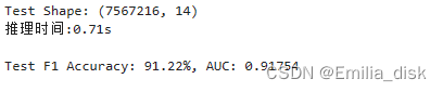
print('推理时间:{:.2f}s'.format(end-start))
print("\nTest F1 Accuracy: {:.2f}%, AUC: {:.5f}".format(xgb_f1*100, xgb_auc))最后测试数据的推理时间为0.71s,F1分数为91.22%。
总结:
通过本次课程的学习,我对数据分析和机器学习相关领域有了更多的理解,对boosting有了更深刻的学习。通过Intel AI Analytics Toolkit让我更加顺利完成了本次课程,了解了oneAPI在AI领域的强大作用,对深度学习和机器学习领域的深度支持让我在完成项目时更加轻松。


 被折叠的 条评论
为什么被折叠?
被折叠的 条评论
为什么被折叠?
 到【灌水乐园】发言


