SPPNet(Spatial Pyramid Pooling in Deep Convolutional Networks for Visual Recognition)

1.Issue：

• R-CNN repeatedly applies DCNN to about 2k candidate windows per image, which is time-consuming.
• The requirement of fixed-size input image is artificial and may reduce the recognition accuracy for the images or sub-images of an arbitrary size/scale.(The cropped region may not contain the entire object, while the warped content may result in unwanted geometric distortion)

2.Innovation:

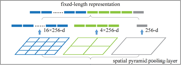
• Replace the last pooling layer with a Spatial Pyramid Pooling
  Layer(Dynamic pooling kernel size and stride) to overlook the
  fixed-size constraint coming from the fully-connected layers.
• Train each full epoch with regions of fixed scale and switch to
  another scale for the next full epoch.(Multi-size training converges
  just as the traditional single-size training, and lead to better
  testing accuracy).
• Run the convolutional layers only once on the entire image.(get conv5
  feature maps from the entire image → map each window to feature maps → apply SPP to regions of feature maps corresponding to candidate windows)

3.Implementation of n-level pyramid:

→ Input: conv5_out: (batch_size, chs, h, w)
  batch_size = conv5_out.shape[0]
  h, w = conv5_out.shape[2], conv5_out.shape[3]
  for i in range(len(spp_out_size)):  # spp_out_size: [(1, 1), (2, 2), ...]
      window_h = math.ceil(h / spp_out_size[i][0])
      window_w = math.ceil(w / spp_out_size[i][1])
      stride_h = math.floor(h / spp_out_size[i][0])
      stride_w = math.floor(w / spp_out_size[i][0])
      max_pooling = nn.MaxPool2d(kernel_size=(window_h, window_w), stride=(stride_h, stride_w))
      x = max_pooling(conv5_out)
      if i == 0:
          spp = torch.reshape(x, (batch_size, -1))
      else:
          spp = torch.cat((spp, torch.reshape(x, (batch_size, -1))), dim=1)
  → Output: spp  #  (batch_size, chs * (1 * 1 + 2 * 2 + ...))

4.Map a window to feature maps:

4.Project the corner point of a window onto a pixel in the feature maps, such that this corner point in the image domain is closest to the center of the receptive field of that feature map pixel. To simplify the complication caused by the padding of all convolutional and pooling layers, during deployment, pad ⌊p/2⌋pixels for a layer with a filter size of p. As such, for a response centered at (x’, y’), its effective receptive field in the image domain is centered at (x, y) = (Sx’, Sy’) where S is the product of all previous stride. Given a window in the image in the image domain, we project the left(top) boundary by: x’ = ⌊x/S⌋+ 1 and the right(bottom) boundary x’= ⌊x/S⌋- 1. If the padding is not ⌊p/2⌋, add a proper offset to x.

5.Weakness of SPPNet:

• Training is a multi-stage pipeline and features to train SVMs and
  bounding-box regressors are written to disk.
• The fine-tuning algorithm cannot update the convolutional layers that
  precede the SPP because back-propagation through the SPP layer is
  highly inefficient when each training sample(RoI) comes from a
  different image, stemming from that each RoI may have a very large
  receptive field, often spanning the entire input image, causing the
  training inputs are large since the forward pass must process the
  entire receptive field.