


pytorch实现
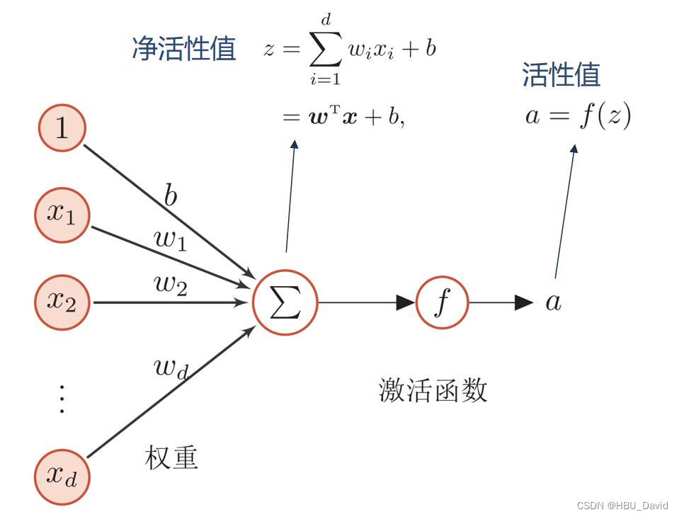
4.1 神经元
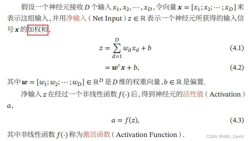
4.1.1 净活性值
使用pytorch计算一组输入的净活性值z
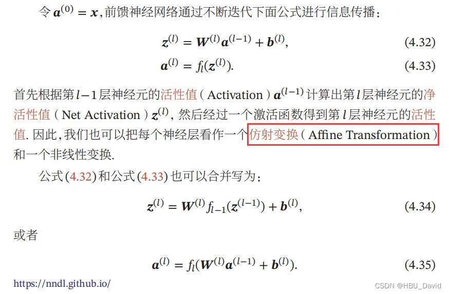
净活性值z经过一个非线性函数f(·)后,得到神经元的活性值a
使用pytorch计算一组输入的净活性值,代码参考paddle例题:
import paddle

# 2个特征数为5的样本
X = paddle.rand(shape=[2, 5])

# 含有5个参数的权重向量
w = paddle.rand(shape=[5, 1])
# 偏置项
b = paddle.rand(shape=[1, 1])

# 使用'paddle.matmul'实现矩阵相乘
z = paddle.matmul(X, w) + b
print("input X:", X)
print("weight w:", w, "\nbias b:", b)
print("output z:", z)
在飞桨中,可以使用nn.Linear完成输入张量的上述变换。
在pytorch中学习相应函数torch.nn.Linear(features_in, features_out, bias=False)。
实现上面的例子,完成代码,进一步深入研究torch.nn.Linear()的使用。
import torch

# 2个特征数为5的样本
X = torch.rand(size=[2, 5])

# 含有5个参数的权重向量
w = torch.rand(size=[5, 1])
# 偏置项
b = torch.rand(size=[1, 1])

# 使用'paddle.matmul'实现矩阵相乘
z = torch.matmul(X, w) + b
print("input X:", X)
print("weight w:", w, "\nbias b:", b)
print("output z:", z)


fc = torch.nn.Linear(5,1)
z = fc(X)

print('m.weight.shape:\n ', fc.weight)
print('m.bias.shape:\n', fc.bias)
print('output.shape:\n', z.shape)
print('output:\n', z)
input X: tensor([[0.8348, 0.0965, 0.5675, 0.6866, 0.0386],
        [0.6098, 0.8196, 0.6592, 0.1052, 0.0593]])
weight w: tensor([[0.2700],
        [0.4832],
        [0.9904],
        [0.6179],
        [0.5249]])
bias b: tensor([[0.6089]])
output z: tensor([[1.8875],
        [1.9185]])
m.weight.shape:
  Parameter containing:
tensor([[-0.1820,  0.2593, -0.1644, -0.2548, -0.0099]], requires_grad=True)
m.bias.shape:
 Parameter containing:
tensor([-0.2644], requires_grad=True)
output.shape:
 torch.Size([2, 1])
output:
 tensor([[-0.6599],
        [-0.2985]], grad_fn=<AddmmBackward0>)
【思考题】加权求和与仿射变换之间有什么区别和联系?
平移(translation)和旋转(rotation)顾名思义,两者的组合称之为欧式变换(Euclidean transformation)或刚体变换(rigid transformation);
放缩(scaling)可进一步分为uniform scaling和non-uniform scaling,前者每个坐标轴放缩系数相同(各向同性),后者不同;如果放缩系数为负,则会叠加上反射(reflection)——reflection可以看成是特殊的scaling;
刚体变换+uniform scaling 称之为,相似变换(similarity transformation),即平移+旋转+各向同性的放缩;
剪切变换(shear mapping)将所有点沿某一指定方向成比例地平移,语言描述不如上面图示直观。
4.1.2 激活函数
激活函数通常为非线性函数,可以增强神经网络的表示能力和学习能力。
常用的激活函数有S型函数和ReLU函数。
4.1.2.1 Sigmoid 型函数
常用的 Sigmoid 型函数有 Logistic 函数和 Tanh 函数。
使用python实现并可视化“Logistic函数、Tanh函数”
在飞桨中,可以通过调用paddle.nn.functional.sigmoid和paddle.nn.functional.tanh实现对张量的Logistic和Tanh计算。在pytorch中找到相应函数并测试。
import torch
import matplotlib.pyplot as plt

# Logistic函数
def logistic(z):
    return 1.0 / (1.0 + torch.exp(-z))

# Tanh函数
def tanh(z):
    return (torch.exp(z) - torch.exp(-z)) / (torch.exp(z) + torch.exp(-z))

# 在[-10,10]的范围内生成10000个输入值,用于绘制函数曲线
z = torch.linspace(-10, 10, 10000)

plt.figure()
plt.plot(z.tolist(), logistic(z).tolist(), color='#e4007f', label="Logistic Function")
plt.plot(z.tolist(), tanh(z).tolist(), color='#f19ec2', linestyle ='--', label="Tanh Function")

ax = plt.gca() # 获取轴,默认有4个
# 隐藏两个轴,通过把颜色设置成none
ax.spines['top'].set_color('none')
ax.spines['right'].set_color('none')
# 调整坐标轴位置
ax.spines['left'].set_position(('data',0))
ax.spines['bottom'].set_position(('data',0))
plt.legend(loc='lower right', fontsize='large')

plt.savefig('fw-logistic-tanh.pdf')
plt.show()

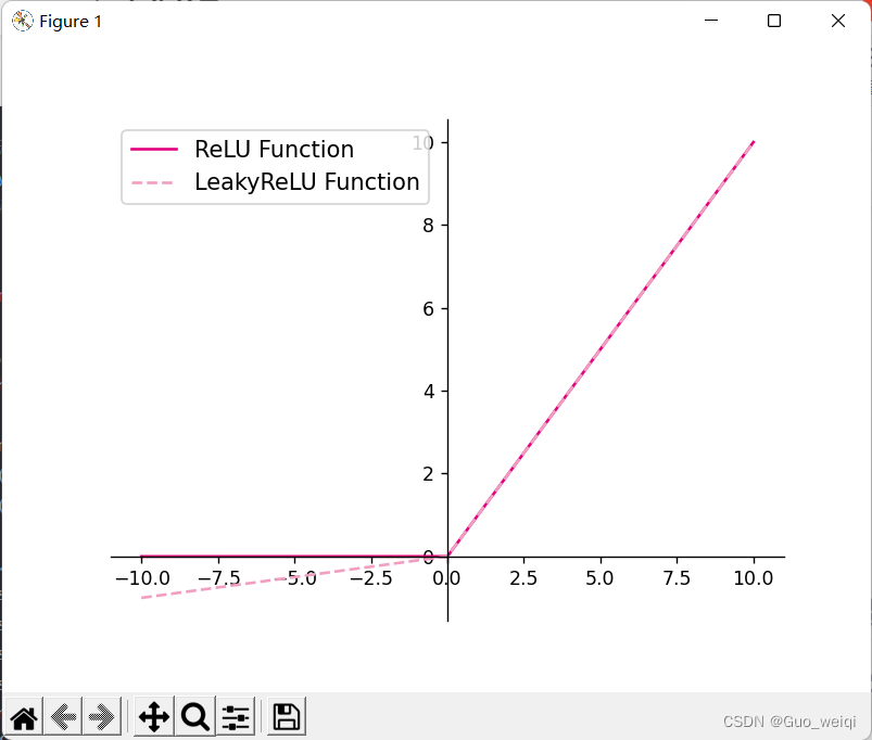
4.1.2.2 ReLU型函数
常见的ReLU函数有ReLU和带泄露的ReLU(Leaky ReLU)
使用python实现并可视化可视化“ReLU、带泄露的ReLU的函数”
在飞桨中,可以通过调用paddle.nn.functional.relu和paddle.nn.functional.leaky_relu完成ReLU与带泄露的ReLU的计算。在pytorch中找到相应函数并测试。
import torch
import matplotlib.pyplot as plt

# ReLU
def relu(z):
    return torch.maximum(z, torch.tensor(0.))

# 带泄露的ReLU
def leaky_relu(z, negative_slope=0.1):
    # 当前版本paddle暂不支持直接将bool类型转成int类型,因此调用了paddle的cast函数来进行显式转换
    a1 = (torch.as_tensor((z > 0), dtype=torch.float32) * z)
    a2 = (torch.as_tensor((z <= 0), dtype=torch.float32) * (negative_slope * z))
    return a1 + a2

# 在[-10,10]的范围内生成一系列的输入值,用于绘制relu、leaky_relu的函数曲线
z = torch.linspace(-10, 10, 10000)

plt.figure()
plt.plot(z.tolist(), relu(z).tolist(), color="#e4007f", label="ReLU Function")
plt.plot(z.tolist(), leaky_relu(z).tolist(), color="#f19ec2", linestyle="--", label="LeakyReLU Function")

ax = plt.gca()
ax.spines['top'].set_color('none')
ax.spines['right'].set_color('none')
ax.spines['left'].set_position(('data',0))
ax.spines['bottom'].set_position(('data',0))
plt.legend(loc='upper left', fontsize='large')
plt.savefig('fw-relu-leakyrelu.pdf')
plt.show()
动手实现《神经网络与深度学习》4.1节中提到的其他激活函数:
Hard-Logistic、Hard-Tanh、ELU、Softplus、Swish等。(选做)
4.2 基于前馈神经网络的二分类任务
4.2.1 数据集构建
使用第3.1.1节中构建的二分类数据集:Moon1000数据集,其中训练集640条、验证集160条、测试集200条。该数据集的数据是从两个带噪音的弯月形状数据分布中采样得到,每个样本包含2个特征。
import math
import torch
def make_moons(n_samples=1000, shuffle=True, noise=None):
"""
生成带噪音的弯月形状数据
输入:
- n_samples:数据量大小,数据类型为int
- shuffle:是否打乱数据,数据类型为bool
- noise:以多大的程度增加噪声,数据类型为None或float,noise为None时表示不增加噪声
输出:
- X:特征数据,shape=[n_samples,2]
- y:标签数据, shape=[n_samples]
"""
n_samples_out = n_samples // 2
n_samples_in = n_samples - n_samples_out
# 采集第1类数据,特征为(x,y)
# 使用'paddle.linspace'在0到pi上均匀取n_samples_out个值
# 使用'paddle.cos'计算上述取值的余弦值作为特征1,使用'paddle.sin'计算上述取值的正弦值作为特征2
outer_circ_x = torch.cos(torch.linspace(0, math.pi, n_samples_out))
outer_circ_y = torch.sin(torch.linspace(0, math.pi, n_samples_out))
inner_circ_x = 1 - torch.cos(torch.linspace(0, math.pi, n_samples_in))
inner_circ_y = 0.5 - torch.sin(torch.linspace(0, math.pi, n_samples_in))
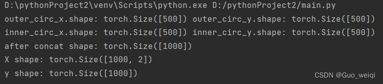
print('outer_circ_x.shape:', outer_circ_x.shape, 'outer_circ_y.shape:', outer_circ_y.shape)
print('inner_circ_x.shape:', inner_circ_x.shape, 'inner_circ_y.shape:', inner_circ_y.shape)
# 使用'paddle.concat'将两类数据的特征1和特征2分别延维度0拼接在一起,得到全部特征1和特征2
# 使用'paddle.stack'将两类特征延维度1堆叠在一起
X = torch.stack(
[torch.cat([outer_circ_x, inner_circ_x]),
torch.cat([outer_circ_y, inner_circ_y])],
dim=1
)
print('after concat shape:', torch.cat([outer_circ_x, inner_circ_x]).shape)
print('X shape:', X.shape)
# 使用'paddle. zeros'将第一类数据的标签全部设置为0
# 使用'paddle. ones'将第一类数据的标签全部设置为1
y = torch.cat(
[torch.zeros(size=[n_samples_out]), torch.ones(size=[n_samples_in])]
)
print('y shape:', y.shape)
# 如果shuffle为True,将所有数据打乱
if shuffle:
# 使用'paddle.randperm'生成一个数值在0到X.shape[0],随机排列的一维Tensor做索引值,用于打乱数据
idx = torch.randperm(X.shape[0])
X = X[idx]
y = y[idx]
# 如果noise不为None,则给特征值加入噪声
if noise is not None:
# 使用'paddle.normal'生成符合正态分布的随机Tensor作为噪声,并加到原始特征上
X += torch.normal(mean=0.0, std=noise, size=X.shape)
return X, y
n_samples = 1000
X, y = make_moons(n_samples=n_samples, shuffle=True, noise=0.5)
num_train = 640
num_dev = 160
num_test = 200
X_train, y_train = X[:num_train], y[:num_train]
X_dev, y_dev = X[num_train:num_train + num_dev], y[num_train:num_train + num_dev]
X_test, y_test = X[num_train + num_dev:], y[num_train + num_dev:]
y_train = y_train.reshape([-1, 1])
y_dev = y_dev.reshape([-1, 1])
y_test = y_test.reshape([-1, 1])
4.2.2 模型构建
为了更高效的构建前馈神经网络,我们先定义每一层的算子,然后再通过算子组合构建整个前馈神经网络。
4.2.2.1 线性层算子
# 实现线性层算子
class Linear(Op):
    def __init__(self, input_size, output_size, name, weight_init=torch.normal, bias_init=torch.zeros):
        """
        输入:
            - input_size:输入数据维度
            - output_size:输出数据维度
            - name:算子名称
            - weight_init:权重初始化方式,默认使用'paddle.standard_normal'进行标准正态分布初始化
            - bias_init:偏置初始化方式,默认使用全0初始化
        """

        self.params = {}
        # 初始化权重
        self.params['W'] = weight_init([input_size, output_size])
        # 初始化偏置
        self.params['b'] = bias_init([1, output_size])
        self.inputs = None

        self.name = name

    def forward(self, inputs):
        """
        输入:
            - inputs:shape=[N,input_size], N是样本数量
        输出:
            - outputs:预测值,shape=[N,output_size]
        """
        self.inputs = inputs

        outputs = torch.matmul(self.inputs, self.params['W']) + self.params['b']
        return outputs
4.2.2.2 Logistic算子(激活函数)
class Logistic(Op):
    def __init__(self):
        self.inputs = None
        self.outputs = None

    def forward(self, inputs):
        """
        输入:
            - inputs: shape=[N,D]
        输出:
            - outputs:shape=[N,D]
        """
        outputs = 1.0 / (1.0 + torch.exp(-inputs))
        self.outputs = outputs
        return outputs
4.2.2.3 层的串行组合
实现一个两层的用于二分类任务的前馈神经网络,选用Logistic作为激活函数,可以利用上面实现的线性层和激活函数算子来组装
实例化一个两层的前馈网络,令其输入层维度为5,隐藏层维度为10,输出层维度为1。
并随机生成一条长度为5的数据输入两层神经网络,观察输出结果。
# 实现一个两层前馈神经网络
class Model_MLP_L2(Op):
    def __init__(self, input_size, hidden_size, output_size):
        """
        输入:
            - input_size:输入维度
            - hidden_size:隐藏层神经元数量
            - output_size:输出维度
        """
        self.fc1 = Linear(input_size, hidden_size, name="fc1")
        self.act_fn1 = Logistic()
        self.fc2 = Linear(hidden_size, output_size, name="fc2")
        self.act_fn2 = Logistic()

    def __call__(self, X):
        return self.forward(X)

    def forward(self, X):
        """
        输入:
            - X:shape=[N,input_size], N是样本数量
        输出:
            - a2:预测值,shape=[N,output_size]
        """
        z1 = self.fc1(X)
        a1 = self.act_fn1(z1)
        z2 = self.fc2(a1)
        a2 = self.act_fn2(z2)
        return a2
model = Model_MLP_L2(input_size=5, hidden_size=10, output_size=1)
# 随机生成1条长度为5的数据
X = torch.rand(size=[1, 5])
result = model(X)
print ("result: ", result)


result:  tensor([[0.4737]])
4.2.3 损失函数
二分类交叉熵损失函数见第三章
import op
class BinaryCrossEntropyLoss(op.Op):
    def __init__(self):
        self.predicts = None
        self.labels = None
        self.num = None

    def __call__(self, predicts, labels):
        return self.forward(predicts, labels)

    def forward(self, predicts, labels):
        """
        输入:
            - predicts:预测值,shape=[N, 1],N为样本数量
            - labels:真实标签,shape=[N, 1]
        输出:
            - 损失值:shape=[1]
        """
        self.predicts = predicts
        self.labels = labels
        self.num = self.predicts.shape[0]
        loss = -1. / self.num * (torch.matmul(self.labels.t(), torch.log(self.predicts)) + torch.matmul((1-self.labels.t()), torch.log(1-self.predicts)))
        loss = torch.squeeze(loss, dim=1)
        return loss

# 测试一下
# 生成一组长度为3,值为1的标签数据
labels = torch.ones(size=[3,1])
# 计算风险函数
bce_loss = BinaryCrossEntropyLoss()
print(bce_loss(outputs, labels))


tensor([0.6931])
4.2.4 模型优化
神经网络的层数通常比较深,其梯度计算和上一章中的线性分类模型的不同的点在于:
线性模型通常比较简单可以直接计算梯度,而神经网络相当于一个复合函数,需要利用链式法则进行反向传播来计算梯度。
4.2.4.1 反向传播算法
第1步是前向计算,可以利用算子的forward()方法来实现;
第2步是反向计算梯度,可以利用算子的backward()方法来实现;
第3步中的计算参数梯度也放到backward()中实现,更新参数放到另外的优化器中专门进行。
4.2.4.2 损失函数
二分类交叉熵损失函数
实现损失函数的backward()
# 实现交叉熵损失函数
class BinaryCrossEntropyLoss(Op):
    def __init__(self, model):
        self.predicts = None
        self.labels = None
        self.num = None

        self.model = model

    def __call__(self, predicts, labels):
        return self.forward(predicts, labels)

    def forward(self, predicts, labels):
        """
        输入:
            - predicts:预测值,shape=[N, 1],N为样本数量
            - labels:真实标签,shape=[N, 1]
        输出:
            - 损失值:shape=[1]
        """
        self.predicts = predicts
        self.labels = labels
        self.num = self.predicts.shape[0]
        loss = -1. / self.num * (torch.matmul(self.labels.t(), torch.log(self.predicts))
                                 + torch.matmul((1 - self.labels.t()), torch.log(1 - self.predicts)))

        loss = torch.squeeze(loss, axis=1)
        return loss

    def backward(self):
        # 计算损失函数对模型预测的导数
        loss_grad_predicts = -1.0 * (self.labels / self.predicts -
                                     (1 - self.labels) / (1 - self.predicts)) / self.num

        # 梯度反向传播
        self.model.backward(loss_grad_predicts)
4.2.4.3 Logistic算子
为Logistic算子增加反向函数
class Logistic(Op):
    def __init__(self):
        self.inputs = None
        self.outputs = None
        self.params = None

    def forward(self, inputs):
        outputs = 1.0 / (1.0 + torch.exp(-inputs))
        self.outputs = outputs
        return outputs

    def backward(self, grads):
        # 计算Logistic激活函数对输入的导数
        outputs_grad_inputs = torch.multiply(self.outputs, (1.0 - self.outputs))
        return torch.multiply(grads,outputs_grad_inputs)
4.2.4.4 线性层
线性层输入的梯度
计算线性层参数的梯度
class Linear(Op):
    def __init__(self, input_size, output_size, name, weight_init=torch.normal, bias_init=torch.zeros):
        self.params = {}
        self.params['W'] = weight_init(mean=0.,std=1.,size=[input_size,output_size])
        self.params['b'] = bias_init([1, output_size])

        self.inputs = None
        self.grads = {}

        self.name = name

    def forward(self, inputs):
        self.inputs = inputs
        outputs = torch.matmul(self.inputs, self.params['W']) + self.params['b']
        return outputs

    def backward(self, grads):
        """
        输入:
            - grads:损失函数对当前层输出的导数
        输出:
            - 损失函数对当前层输入的导数
        """
        self.grads['W'] = torch.matmul(self.inputs.T, grads)
        self.grads['b'] = torch.sum(grads, axis=0)

        # 线性层输入的梯度
        return torch.matmul(grads, self.params['W'].T)
4.2.4.5 整个网络
实现完整的两层神经网络的前向和反向计算
class Model_MLP_L2(Op):
    def __init__(self, input_size, hidden_size, output_size):
        # 线性层
        self.fc1 = Linear(input_size, hidden_size, name="fc1")
        # Logistic激活函数层
        self.act_fn1 = Logistic()
        self.fc2 = Linear(hidden_size, output_size, name="fc2")
        self.act_fn2 = Logistic()

        self.layers = [self.fc1, self.act_fn1, self.fc2, self.act_fn2]

    def __call__(self, X):
        return self.forward(X)

    # 前向计算
    def forward(self, X):
        z1 = self.fc1(X)
        a1 = self.act_fn1(z1)
        z2 = self.fc2(a1)
        a2 = self.act_fn2(z2)
        return a2

    # 反向计算
    def backward(self, loss_grad_a2):
        loss_grad_z2 = self.act_fn2.backward(loss_grad_a2)
        loss_grad_a1 = self.fc2.backward(loss_grad_z2)
        loss_grad_z1 = self.act_fn1.backward(loss_grad_a1)
        loss_grad_inputs = self.fc1.backward(loss_grad_z1)
4.2.4.6 优化器
在计算好神经网络参数的梯度之后,我们将梯度下降法中参数的更新过程实现在优化器中。
与第3章中实现的梯度下降优化器SimpleBatchGD不同的是,此处的优化器需要遍历每层,对每层的参数分别做更新。
class BatchGD(Optimizer):
    def __init__(self, init_lr, model):
        super(BatchGD, self).__init__(init_lr=init_lr, model=model)

    def step(self):
        # 参数更新
        for layer in self.model.layers: # 遍历所有层
            if isinstance(layer.params, dict):
                for key in layer.params.keys():
                    layer.params[key] = layer.params[key] - self.init_lr * layer.grads[key]
4.2.5 完善Runner类:RunnerV2_1
支持自定义算子的梯度计算,在训练过程中调用self.loss_fn.backward()从损失函数开始反向计算梯度;
每层的模型保存和加载,将每一层的参数分别进行保存和加载。
class RunnerV2_1(object):
    def __init__(self, model, optimizer, metric, loss_fn, **kwargs):
        self.model = model
        self.optimizer = optimizer
        self.loss_fn = loss_fn
        self.metric = metric

        # 记录训练过程中的评估指标变化情况
        self.train_scores = []
        self.dev_scores = []

        # 记录训练过程中的评价指标变化情况
        self.train_loss = []
        self.dev_loss = []

    def train(self, train_set, dev_set, **kwargs):
        # 传入训练轮数,如果没有传入值则默认为0
        num_epochs = kwargs.get("num_epochs", 0)
        # 传入log打印频率,如果没有传入值则默认为100
        log_epochs = kwargs.get("log_epochs", 100)

        # 传入模型保存路径
        save_dir = kwargs.get("save_dir", None)

        # 记录全局最优指标
        best_score = 0
        # 进行num_epochs轮训练
        for epoch in range(num_epochs):
            X, y = train_set
            # 获取模型预测
            logits = self.model(X)
            # 计算交叉熵损失
            trn_loss = self.loss_fn(logits, y)  # return a tensor

            self.train_loss.append(trn_loss.item())
            # 计算评估指标
            trn_score = self.metric(logits, y).item()
            self.train_scores.append(trn_score)

            self.loss_fn.backward()

            # 参数更新
            self.optimizer.step()

            dev_score, dev_loss = self.evaluate(dev_set)
            # 如果当前指标为最优指标,保存该模型
            if dev_score > best_score:
                print(f"[Evaluate] best accuracy performence has been updated: {best_score:.5f} --> {dev_score:.5f}")
                best_score = dev_score
                if save_dir:
                    self.save_model(save_dir)

            if log_epochs and epoch % log_epochs == 0:
                print(f"[Train] epoch: {epoch}/{num_epochs}, loss: {trn_loss.item()}")

    def evaluate(self, data_set):
        X, y = data_set
        # 计算模型输出
        logits = self.model(X)
        # 计算损失函数
        loss = self.loss_fn(logits, y).item()
        self.dev_loss.append(loss)
        # 计算评估指标
        score = self.metric(logits, y).item()
        self.dev_scores.append(score)
        return score, loss

    def predict(self, X):
        return self.model(X)

    def save_model(self, save_dir):
        # 对模型每层参数分别进行保存,保存文件名称与该层名称相同
        for layer in self.model.layers:  # 遍历所有层
            if isinstance(layer.params, dict):
               torch.save(layer.params, os.path.join(save_dir, layer.name+".pdparams"))

    def load_model(self, model_dir):
        # 获取所有层参数名称和保存路径之间的对应关系
        model_file_names = os.listdir(model_dir)
        name_file_dict = {}
        for file_name in model_file_names:
            name = file_name.replace(".pdparams", "")
            name_file_dict[name] = os.path.join(model_dir, file_name)

        # 加载每层参数
        for layer in self.model.layers:  # 遍历所有层
            if isinstance(layer.params, dict):
                name = layer.name
                file_path = name_file_dict[name]
                layer.params = torch.load(file_path)
4.2.6 模型训练
使用训练集和验证集进行模型训练,共训练2000个epoch。评价指标为accuracy。
epoch_num = 1000

model_saved_dir = 'D:\\apps\python\pytorch\save'

# 输入层维度为2
input_size = 2
# 隐藏层维度为5
hidden_size = 5
# 输出层维度为1
output_size = 1

# 定义网络
model = Model_MLP_L2(input_size=input_size, hidden_size=hidden_size, output_size=output_size)

# 损失函数
loss_fn = BinaryCrossEntropyLoss(model)

# 优化器
learning_rate = 0.2
optimizer = BatchGD(learning_rate, model)

# 评价方法
metric = accuracy

# 实例化RunnerV2_1类,并传入训练配置
runner = RunnerV2_1(model, optimizer, metric, loss_fn)

runner.train([X_train, y_train], [X_dev, y_dev], num_epochs=epoch_num, log_epochs=50, save_dir=model_saved_dir)


[Evaluate] best accuracy performence has been updated: 0.00000 --> 0.16875
[Train] epoch: 0/1000, loss: 0.7350932955741882
[Evaluate] best accuracy performence has been updated: 0.16875 --> 0.17500
[Evaluate] best accuracy performence has been updated: 0.17500 --> 0.18750
[Evaluate] best accuracy performence has been updated: 0.18750 --> 0.20000
[Evaluate] best accuracy performence has been updated: 0.20000 --> 0.21250
[Evaluate] best accuracy performence has been updated: 0.21250 --> 0.22500
[Evaluate] best accuracy performence has been updated: 0.22500 --> 0.25000
[Evaluate] best accuracy performence has been updated: 0.25000 --> 0.31250
[Evaluate] best accuracy performence has been updated: 0.31250 --> 0.37500
[Evaluate] best accuracy performence has been updated: 0.37500 --> 0.43750
[Evaluate] best accuracy performence has been updated: 0.43750 --> 0.46250
[Evaluate] best accuracy performence has been updated: 0.46250 --> 0.48125
[Evaluate] best accuracy performence has been updated: 0.48125 --> 0.49375
[Evaluate] best accuracy performence has been updated: 0.49375 --> 0.51250
[Evaluate] best accuracy performence has been updated: 0.51250 --> 0.55625
[Evaluate] best accuracy performence has been updated: 0.55625 --> 0.60625
[Evaluate] best accuracy performence has been updated: 0.60625 --> 0.61875
[Evaluate] best accuracy performence has been updated: 0.61875 --> 0.63750
[Evaluate] best accuracy performence has been updated: 0.63750 --> 0.65000
[Evaluate] best accuracy performence has been updated: 0.65000 --> 0.66250
[Evaluate] best accuracy performence has been updated: 0.66250 --> 0.66875
[Evaluate] best accuracy performence has been updated: 0.66875 --> 0.67500
[Evaluate] best accuracy performence has been updated: 0.67500 --> 0.68125
[Evaluate] best accuracy performence has been updated: 0.68125 --> 0.68750
[Evaluate] best accuracy performence has been updated: 0.68750 --> 0.69375
[Evaluate] best accuracy performence has been updated: 0.69375 --> 0.70000
[Evaluate] best accuracy performence has been updated: 0.70000 --> 0.71250
[Evaluate] best accuracy performence has been updated: 0.71250 --> 0.71875
[Train] epoch: 50/1000, loss: 0.664116382598877
[Evaluate] best accuracy performence has been updated: 0.71875 --> 0.72500
[Evaluate] best accuracy performence has been updated: 0.72500 --> 0.73750
[Evaluate] best accuracy performence has been updated: 0.73750 --> 0.74375
[Evaluate] best accuracy performence has been updated: 0.74375 --> 0.75000
[Evaluate] best accuracy performence has been updated: 0.75000 --> 0.76250
[Evaluate] best accuracy performence has been updated: 0.76250 --> 0.76875
[Evaluate] best accuracy performence has been updated: 0.76875 --> 0.78125
[Evaluate] best accuracy performence has been updated: 0.78125 --> 0.79375
[Evaluate] best accuracy performence has been updated: 0.79375 --> 0.80625
[Evaluate] best accuracy performence has been updated: 0.80625 --> 0.81250
[Train] epoch: 100/1000, loss: 0.5949881076812744
[Evaluate] best accuracy performence has been updated: 0.81250 --> 0.81875
[Evaluate] best accuracy performence has been updated: 0.81875 --> 0.82500
[Evaluate] best accuracy performence has been updated: 0.82500 --> 0.83125
[Evaluate] best accuracy performence has been updated: 0.83125 --> 0.83750
[Train] epoch: 150/1000, loss: 0.5277273058891296
[Train] epoch: 200/1000, loss: 0.485870361328125
[Train] epoch: 250/1000, loss: 0.46499910950660706
[Train] epoch: 300/1000, loss: 0.4550503194332123
[Train] epoch: 350/1000, loss: 0.45022842288017273
[Train] epoch: 400/1000, loss: 0.44782382249832153
[Train] epoch: 450/1000, loss: 0.44659096002578735
[Evaluate] best accuracy performence has been updated: 0.83750 --> 0.84375
[Train] epoch: 500/1000, loss: 0.44594064354896545
[Evaluate] best accuracy performence has been updated: 0.84375 --> 0.85000
[Evaluate] best accuracy performence has been updated: 0.85000 --> 0.85625
[Train] epoch: 550/1000, loss: 0.44558531045913696
[Train] epoch: 600/1000, loss: 0.4453815519809723
[Evaluate] best accuracy performence has been updated: 0.85625 --> 0.86250
[Train] epoch: 650/1000, loss: 0.44525671005249023
[Train] epoch: 700/1000, loss: 0.4451737403869629
[Train] epoch: 750/1000, loss: 0.4451136589050293
[Train] epoch: 800/1000, loss: 0.4450666606426239
[Train] epoch: 850/1000, loss: 0.4450274407863617
[Train] epoch: 900/1000, loss: 0.4449935853481293
[Train] epoch: 950/1000, loss: 0.44496336579322815


import matplotlib.pyplot as plt
# 打印训练集和验证集的损失
plt.figure()
plt.plot(range(epoch_num), runner.train_loss, color="#e4007f", label="Train loss")
plt.plot(range(epoch_num), runner.dev_loss, color="#f19ec2", linestyle='--', label="Dev loss")
plt.xlabel("epoch", fontsize='large')
plt.ylabel("loss", fontsize='large')
plt.legend(fontsize='x-large')
plt.show()
#加载训练好的模型
runner.load_model(model_saved_dir)
# 在测试集上对模型进行评价
score, loss = runner.evaluate([X_test, y_test])

4.2.7 性能评价
使用测试集对训练中的最优模型进行评价,观察模型的评价指标。
# 加载训练好的模型
runner.load_model(model_saved_dir)
# 在测试集上对模型进行评价
score, loss = runner.evaluate([X_test, y_test])

print("[Test] score/loss: {:.4f}/{:.4f}".format(score, loss))


import math

# 均匀生成40000个数据点
x1, x2 = torch.meshgrid(torch.linspace(-math.pi, math.pi, 200), torch.linspace(-math.pi, math.pi, 200))
x = torch.stack([torch.flatten(x1), torch.flatten(x2)], dim=1)

# 预测对应类别
y = runner.predict(x)
y = torch.squeeze(torch.as_tensor((y>=0.5),dtype=torch.float32),dim=-1)

# 绘制类别区域
plt.ylabel('x2')
plt.xlabel('x1')
plt.scatter(x[:,0].tolist(), x[:,1].tolist(), c=y.tolist(), cmap=plt.cm.Spectral)

plt.scatter(X_train[:, 0].tolist(), X_train[:, 1].tolist(), marker='*', c=torch.squeeze(y_train,dim=-1).tolist())
plt.scatter(X_dev[:, 0].tolist(), X_dev[:, 1].tolist(), marker='*', c=torch.squeeze(y_dev,dim=-1).tolist())
plt.scatter(X_test[:, 0].tolist(), X_test[:, 1].tolist(), marker='*', c=torch.squeeze(y_test,dim=-1).tolist())


 1754
1754


 被折叠的 条评论
为什么被折叠?
被折叠的 条评论
为什么被折叠?
 到【灌水乐园】发言


