三.线性代数, 运筹学, 组合优化(Combinatorial optimisation)之单纯形法(The Simplex Method)

一. Introduction

The simplex method is a technique for solving general LPs. The basic idea is that we represent the problem as a set of linear equations in variables; all variables are required to be ≥0.

We then use information from the objective function to manipulate these equations, by successively eliminating and back-substituting one variable, until the optimal solution becomes “obvious” (moving between vertices).

We will illustrate the method using our two-variable example, though the method works for any number of variables.

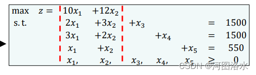
 We first convert to equations in nonnegative variables.

A ≤ constraint can be converted into an equation by introducing a new variable (called a slack variable), e.g.

is equivalent to 

 since x3 just measures the nonnegative amount by which the RHS of (2) exceeds the LHS. Applying this throughout, we get:

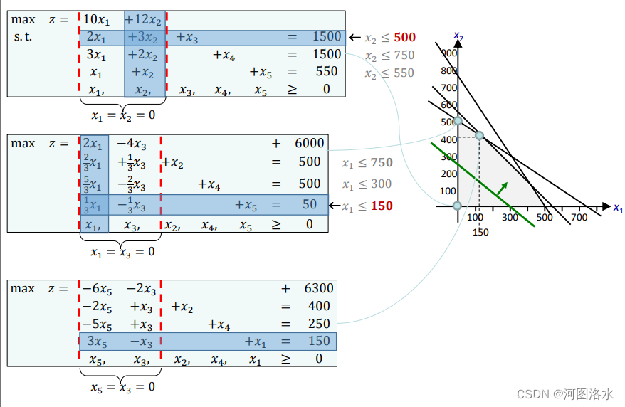
A feasible solution is any solution to the equations which also satisfies xi≥0 for all variables

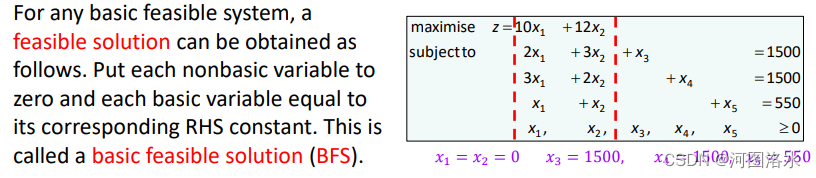
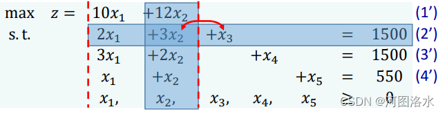
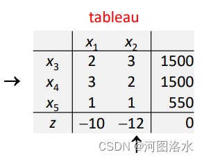
In the simplex method, we always deal with basic sets of equations, i.e. each equation contains a variable with coefficient +1 (the basic variable) which does not appear in any other equation. The other variables are nonbasic. In our example, the set of equations is basic with basic variables x3 , x4 , x5 and nonbasic variables x1 , x2

A basic set of equations is called feasible if all the RHS constants are ≥0. Our set is basic feasible. The simplex method starts with a basic feasible set, and retains basic feasible sets throughout. (If we do not have a basic feasible set to start, then the two-phase simplex method is used.) 

 For any basic feasible system, a feasible solution can be obtained as follows. Put each nonbasic variable to zero and each basic variable equal to its corresponding RHS constant. This is called a basic feasible solution (BFS).

 A feasible solution is any solution to the equations which also satisfies xi≥0 for all variables.

A feasible solution is any solution to the equations which also satisfies xi≥0 for all variables. In the simplex method, we always deal with basic sets of equations, i.e. each equation contains a variable with coefficient +1 (the basic variable) which does not appear in any other equation. The other variables are nonbasic. In our example, the set of equations is basic with basic variables x3 , x4 , x5 and nonbasic variables x1 , x2.

 In the next iteration, the set of equations is also basic with basic variables x2 , x4 , x5 and nonbasic variables x1 , x3 .

 二. Algebraic Simplex Method

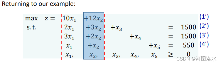
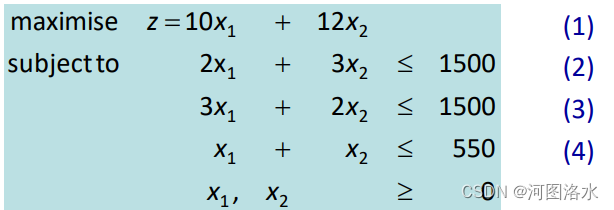
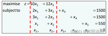
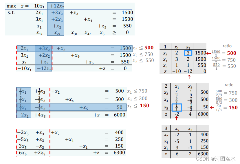
In this BFS, x1= x2= 0, but it appears that z will be larger if either x1 or x2 is made positive (since they both have positive z-coefficients). In the method, we will only change one variable at a time. 

So let us choose x2 , since it has the larger z-coefficient. If we increase x2 from 0, keeping x1= 0, then x3 , x4 , x5 must change according to the reduced set of conditions:

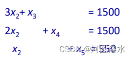
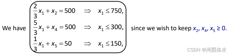
We want to ensure that x3 , x4 , x5 ≥ 0, so observe that 

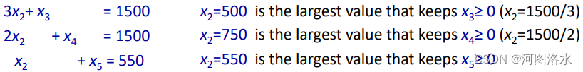
 Thus the largest possible increase of x2 that we can afford keeping x3 , x4 , x5 ≥ 0 is x2 = 500; (for x2 > 500 the value of x3 becomes negative).

 

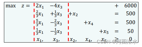
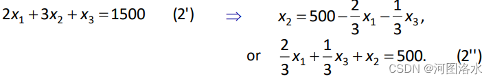
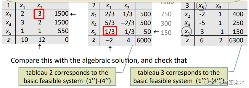
 Thus we now make x1 , x3 the nonbasic variables, by solving for x2 in terms of x1 , x3 and substituting for it, i.e

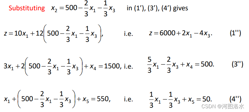
 Thus the new basic feasible system is

 with BFS x1=0, x2=500, x3=0, x4=500, x5=50 and z=6000. (Note that x1 and x3 are now the non-basic variables). So we have increased z from 0 to 6000. We have carried out the first iteration of the simplex method.

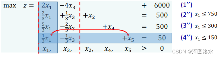
 Since this system is basic feasible, we can continue. This time we see (from z = 2x1 ─ 4x3 + 6000) that we should increase x1 (and we will keep x3=0).

 

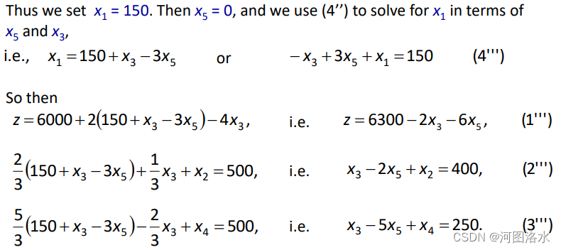
 Thus the new basic feasible system is

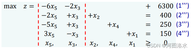
 with BFS x1=150, x2=400, x3=0, x4=250, x5=0 and z=6300

So we have increased z further from 6000 to 6300, and again we have a basic feasible system of equations. We have carried out the second iteration of the simplex method.

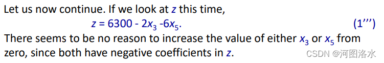
 But, in fact, something much stronger is true. Since we must have x3 , x5 ≥ 0, we see that (1’’’) implies z ≤ 6300.

Thus we know that there can be no feasible solution better than our current BFS, i.e. x1=150, x2=400, x3=0, x4=250, x5=0 and z=6300 is the optimal solution to our original LP problem.

Thus the simplex method has solved this LP problem in two iterations.

The same methodology can be applied to any linear program in any number of variables, provided only that we have a basic feasible system to start the process.

The only problem is that the elimination and substitution steps are cumbersome. Fortunately, we can put the whole process in a convenient tabular format: the contracted simplex tableau.

三. Tableau Simplex Method

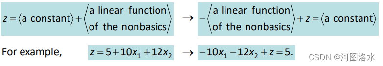
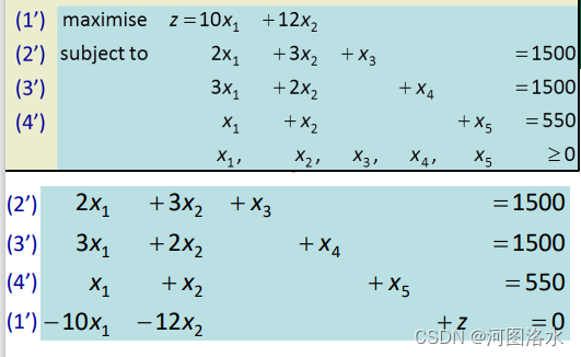
 In order to put the solution process in a convenient tabular format, we first put z in the same form as the other equations in the basic system, i.e.

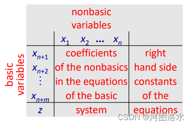
 The tableau for any basic system then has the format:

In each row, the coefficients are multiplied by the variable at the head of the column, and then these terms are added together. The vertical line at the left side represents a “+” and the vertical line at the right side an “=“ in each equation. The z row is separated by a horizontal line to indicate that it is an objective function row.

 `

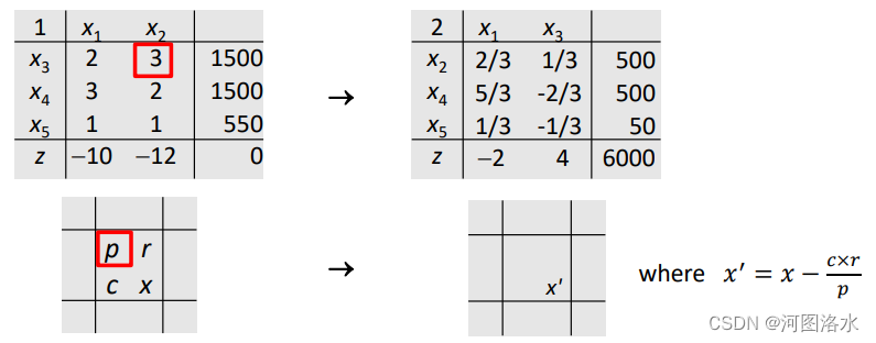
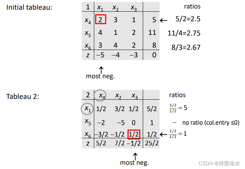
 Notice that, if we are maximizing, it is now the negative coefficients of nonbasics in the z-row which are of interest. We choose the most negative, though any negative would do. This identifies a column of the tableau, called the pivot column.

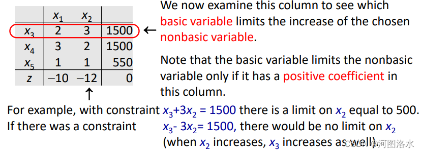
In the simplex tableau, we can determine which basic, becoming zero, limits the chosen nonbasic by the following ratio test:

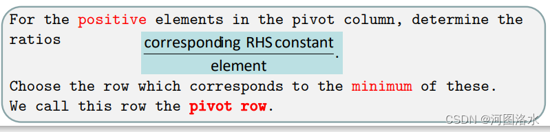
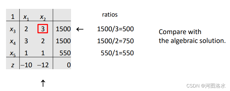
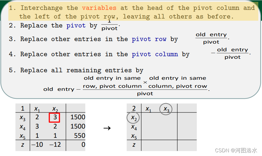
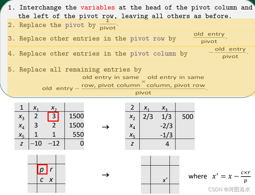
 The boxed element at the intersection of the pivot row and column is called the pivot. ratios Compare with the algebraic solution. The rules for the elimination and back substitution are then as follows.

In a new tableau,

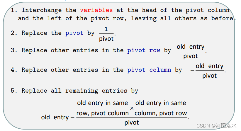
 This is just a systematic way of performing the algebraic elimination and substitution of the variable at the head of the pivot column and the variable at the left of the pivot row.

1.

2.-5.

 

Then

 

compare

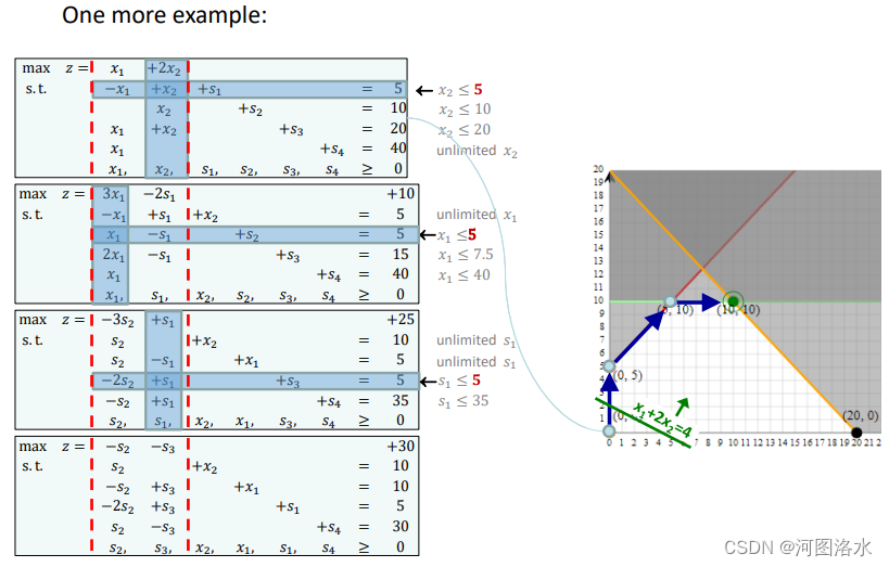
Example:

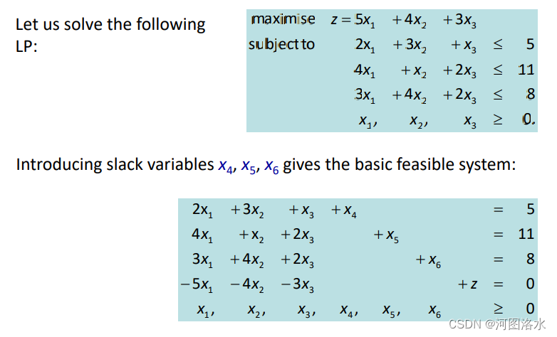
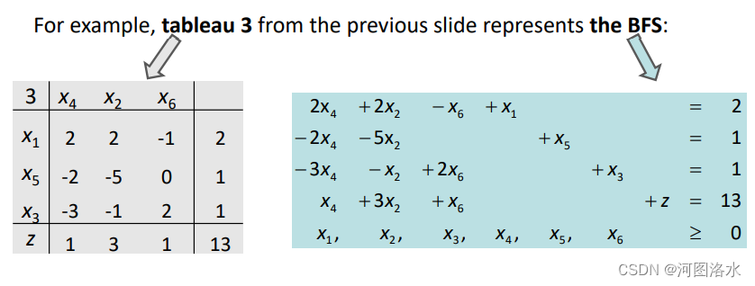
A 3-variable LP in Tableau Format Introducing slack variables x4 , x5 , x6 gives the basic feasible system: , , 0. 3 4 2 8 4 2 11 subjectto 2x 3 5 maximise 5 4 3 1 2 3 1 2 3 1 2 3 1 2 3

 

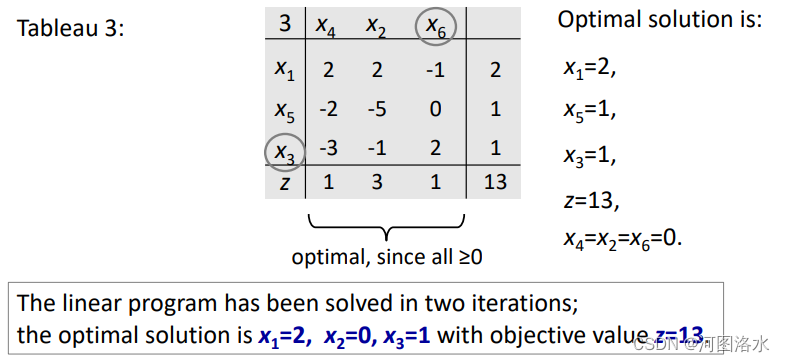
 Notice that we can move between the tableau and the basic feasible system it represents quite easily