计算机视觉（八）：提取Cifar-10数据集的HOG、HSV特征并使用神经网络进行分类

本文链接：https://blog.csdn.net/HHH_ANS/article/details/86297859

1 - 引言

之前我们都是将整张图片输入进行分类，要想进一步提升准确率，我们就必须提取出图片更容易区分的特征，再将这些特征当做特征向量进行分类。在之前我们学了一些常用的图像特征，在这次实验中，我们使用了两种特征

梯度方向直方图（HOG）
颜色直方图（HSV）

为什么选用这两种特征呢？
应为HOG捕捉到的是图像的纹理特征，而忽略了颜色信息，颜色直方图会表示图像的颜色特征而忽略了纹理特征，因此将这两者的特征结合起来可能会得到一个比较好的结果，当然，我们也可以试试选用其他的特征，有可能可以得到更好的效果哦

然后把每张图的梯度方向直方图和颜色直方图特征合并形成我们最后的特征向量，将特征向量输入进神经网络中进行训练，并完成分类。

2 - 具体步骤

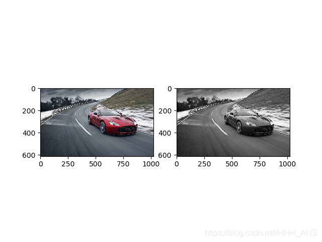
2.1 - RGB彩色图像转化成灰度图

由公式 $i m g = 0.299 * R + 0.587 * G + 0.144 * B$
可得

def rgb2gray(rgb):
    """
    将RGB图片转换成灰度图片：公式img = 0.299 * R + 0.587 * G + 0.144 * B

      输入:
        rgb : RGB 图片
      返回:
        gray : 灰度图片

    """
    return np.dot(rgb[..., :3], [0.299, 0.587, 0.144])

我们可以测试一下

import numpy as np
import matplotlib.pyplot as plt


def rgb2gray(rgb):
    return np.dot(rgb[..., :3], [0.299, 0.587, 0.114])


img = plt.imread('images/car.jpg')
gray = img
plt.imshow(gray, cmap=plt.get_cmap('gray'))
plt.show()

在这里插入图片描述

2.2 - 提取HOG特征

提取HOG特征的步骤如下：

计算水平和垂直方向的梯度
某个像素点的X方向的梯度计算可以通过这个像素点左右两边的像素值的差值的绝对值计算出来，而y方向的梯度可以通过该像素上下两边的像素值的差值的绝对值计算。我们可以使用Sobel算子来计算 $g_x、g_y$
计算梯度的幅值g和方向theta:
$\sqrt{g_x^2+g_y^2}$
$\theta = arctan\frac{g_y}{g_x}$
在88 的网格中计算梯度直方图并且对应到9个bin的直方图中

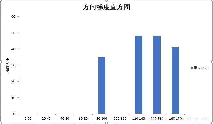
直方图的横轴代表着方向角度
纵轴代表着这88个网格中梯度大小的和
$16 * 16$ 块归一化
用一个 $16 * 16$ 的窗口（4个 $8 * 8$ ），也就是4个 $9 * 1$ 的直方图组合成 $36 * 1$ 的向量，然后做归一化。之后将窗口朝后面挪8个像素，重复这个过程把整张图遍历一遍
对向量使用L2归一化：
$\leftarrow v/\sqrt{||v||^2_2+\varepsilon }(\varepsilon是一个极小的常数，避免分母为0)$
计算HOG特征向量

根据这个思想可以构造函数：

def hog_feature(im):
    """
    计算图片的梯度方向直方图（HOG）特征
         从 skimage.feature.hog 中修改而来
         http://pydoc.net/Python/scikits-image/0.4.2/skimage.feature.hog

       Reference:
         Histograms of Oriented Gradients for Human Detection
         Navneet Dalal and Bill Triggs, CVPR 2005

      Parameters:
        im : 灰度图片或者RBG图片

      Returns:
        feat: HOG 特征

    """

    # 如果图像维数是3维，则转换成灰度图
    if im.ndim == 3:
        image = rgb2gray(im)
    else:
        image = np.at_least_2d(im)

    sx, sy = image.shape  # 图片尺寸
    orientations = 9  # 梯度直方图的数量
    cx, cy = (8, 8)  # 一个单元的像素个数

    gx = np.zeros(image.shape)
    gy = np.zeros(image.shape)
    gx[:, :-1] = np.diff(image, n=1, axis=1)  # compute gradient on x-direction
    gy[:-1, :] = np.diff(image, n=1, axis=0)  # compute gradient on y-direction
    grad_mag = np.sqrt(gx ** 2 + gy ** 2)  # gradient magnitude
    grad_ori = np.arctan2(gy, (gx + 1e-15)) * (180 / np.pi) + 90  # gradient orientation

    n_cellsx = int(np.floor(sx / cx))  # number of cells in x
    n_cellsy = int(np.floor(sy / cy))  # number of cells in y
    # compute orientations integral images
    orientation_histogram = np.zeros((n_cellsx, n_cellsy, orientations))
    for i in range(orientations):
        # create new integral image for this orientation
        # isolate orientations in this range
        temp_ori = np.where(grad_ori < 180 / orientations * (i + 1),
                            grad_ori, 0)
        temp_ori = np.where(grad_ori >= 180 / orientations * i,
                            temp_ori, 0)
        # select magnitudes for those orientations
        cond2 = temp_ori > 0
        temp_mag = np.where(cond2, grad_mag, 0)
        orientation_histogram[:, :, i] = uniform_filter(temp_mag, size=(cx, cy))[int(cx / 2)::cx, int(cy / 2)::cy].T

    return orientation_histogram.ravel()

HOG算法重点
Dalal提出的HOG特征特区的过程，把样本图像分割为若干个像素的单元（cell），把梯度方向平均划分成9个区间（bin）,在每个单元里面对所有像素的梯度方向在各个方向区间进行直方图统计，得到一个9维的特征向量，每相邻的4个单元构成一个块（block），把一个块内的特征向量连起来得到36维的特征向量，用块对样本图像进行扫描，扫描步长为一个单元。最后将所有块的特征串联起来。

例如
一个图片为 $64 * 128$ 的图像，每 $16 * 16$ 的像素组成一个cell,每 $2 * 2$ 个cell组成一个快，因为每个cell有9个特征，所以每个块内又 $4 * 9 = 36$ 个特征，以8个像素为步长，那么，水平方向将有7个扫描窗口，垂直方向有15个扫描窗口，也就是说，64128的图片，总共有367*15 = 3780 个特征

2.3 - 提取HSV特征

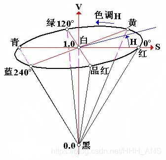
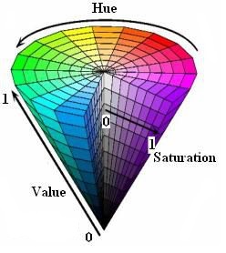
HSV是一种比较直观的颜色模型，所以在许多图像编辑工具中应用比较广泛，这个模型中颜色的参数分别是：色调（H, Hue），饱和度（S,Saturation），明度（V, Value）。

色调H
用角度度量，取值范围为0°～360°，从红色开始按逆时针方向计算，红色为0°，绿色为120°,蓝色为240°。它们的补色是：黄色为60°，青色为180°,品红为300°；

饱和度S
饱和度S表示颜色接近光谱色的程度。一种颜色，可以看成是某种光谱色与白色混合的结果。其中光谱色所占的比例愈大，颜色接近光谱色的程度就愈高，颜色的饱和度也就愈高。饱和度高，颜色则深而艳。光谱色的白光成分为0，饱和度达到最高。通常取值范围为0%～100%，值越大，颜色越饱和。

明度V
明度表示颜色明亮的程度，对于光源色，明度值与发光体的光亮度有关；对于物体色，此值和物体的透射比或反射比有关。通常取值范围为0%（黑）到100%（白）。

在这里插入图片描述

RGB转换HSV公式
设max等于r、g、b中的最大者，min为最小者，对应的HSV空间中的（h,s,v）值为：
$\begin{cases} 0^{\circ} & \text{ if } max=min \\ 60^{\circ} \times \frac{g-b}{max-min} +0^{\circ}& \text{ if } max=r and g \geq b \\ 60^{\circ} \times \frac{g-b}{max-min} +360^{\circ} & \text{ if } max= r and g < b \\ 60^{\circ} \times \frac{g-b}{max-min} +120^{\circ}& \text{ if } max=g \\ 60^{\circ} \times \frac{g-b}{max-min} +240^{\circ}& \text{ if } max=b \end{cases}$

$\begin{cases} 0 & \text{ if } max=0 \\ \frac{max-min}{max}=1-\frac{min}{max} & \text{ if } otherwise \\ \end{cases}$

$v = m a x$

(h在0到 $360^{\circ}$ ,s在0到100%之间，v在0到max之间)

程序如下：

def color_histogram_hsv(im, nbin=10, xmin=0, xmax=255, normalized=True):
    """
    计算HSV颜色特征
    输入：
    - im : H x W x C 的RGB数组
    - nbin : 直方图柱状的数量
    - xmin : 最小像素值（缺省值：0）
    - xmax : 最大像素值（缺省值：255）
    - normalized : 是否归一化（缺省值：True）
    返回：
    - imhist : 图像的颜色直方图

    """
    ndim = im.ndim
    bins = np.linspace(xmin, xmax, nbin + 1)
    hsv = matplotlib.colors.rgb_to_hsv(im / xmax) * xmax
    imhist, bin_edges = np.histogram(hsv[:, :, 0], bins=bins, density=normalized)
    imhist = imhist * np.diff(bin_edges)

    # return histogram
    return imhist

2.4 - 合并特征向量

最后，需要将数据集中每张图片的HOG、HSV的特征向量连接起来，构成一个总的数据集的向量矩阵，维数为（N，F_1+ … + F_k），每一行是单个图像的HOG+HSV的特征向量

def extract_features(imgs, feature_fns, verbose=False):
    """
    给出图片的像素数据和针对单个图片的特征提取函数，可以提取数据集中所有的图片的HOG和HSV特征，并且
    将这些每张图片的特征向量连接起来，存储在一个矩阵中
    输入：
    - imgs : (N,H_x,W_x,C)
    - feature_fns ：K 个特征的列表，第 i 个特征应该输入一个维数为（H，W,D）的图片，然后返回一个
    一维向量，长度为F_i
    - verbose : Boolean；标志量，如果为真则打印特征提取的过程

    返回：
    一个数组，维数为（N，F_1 + ... + F_k），每一行是单个图像的所有特征向量的连接
    """
    num_images = imgs.shape[0]
    if num_images == 0:
        return np.array([])

    # Use the first image to determine feature dimensions
    feature_dims = []
    first_image_features = []
    for feature_fn in feature_fns:
        feats = feature_fn(imgs[0].squeeze())
        assert len(feats.shape) == 1, 'Feature functions must be one-dimensional'
        feature_dims.append(feats.size)
        first_image_features.append(feats)

    # Now that we know the dimensions of the features, we can allocate a single
    # big array to store all features as columns.
    total_feature_dim = sum(feature_dims)
    imgs_features = np.zeros((num_images, total_feature_dim))
    imgs_features[0] = np.hstack(first_image_features).T

    # Extract features for the rest of the images.
    for i in range(1, num_images):
        idx = 0
        for feature_fn, feature_dim in zip(feature_fns, feature_dims):
            next_idx = idx + feature_dim
            imgs_features[i, idx:next_idx] = feature_fn(imgs[i].squeeze())
            idx = next_idx
        if verbose and i % 1000 == 0:
            print('Done extracting features for %d / %d images' % (i, num_images))

    return imgs_features

然后将这个向量矩阵当做神经网络的输入，进行最后的分类，并使用交叉验证得到最佳模型超参数。

import random
import numpy as np
from cs231n.data_utils import load_CIFAR10
import matplotlib.pyplot as plt

from cs231n.features import color_histogram_hsv, hog_feature


def get_CIFAR10_data(num_training=49000, num_validation=1000, num_test=1000):
    # Load the raw CIFAR-10 data
    cifar10_dir = 'cs231n/datasets/cifar-10-batches-py'
    X_train, y_train, X_test, y_test = load_CIFAR10(cifar10_dir)

    # Subsample the data
    mask = range(num_training, num_training + num_validation)
    X_val = X_train[mask]
    y_val = y_train[mask]
    mask = range(num_training)
    X_train = X_train[mask]
    y_train = y_train[mask]
    mask = range(num_test)
    X_test = X_test[mask]
    y_test = y_test[mask]

    return X_train, y_train, X_val, y_val, X_test, y_test


X_train, y_train, X_val, y_val, X_test, y_test = get_CIFAR10_data()

from cs231n.features import *

num_color_bins = 10 # Number of bins in the color histogram
feature_fns = [hog_feature, lambda img: color_histogram_hsv(img, nbin=num_color_bins)]
X_train_feats = extract_features(X_train, feature_fns, verbose=True)
X_val_feats = extract_features(X_val, feature_fns)
X_test_feats = extract_features(X_test, feature_fns)

# Preprocessing: Subtract the mean feature
mean_feat = np.mean(X_train_feats, axis=0, keepdims=True)
X_train_feats -= mean_feat
X_val_feats -= mean_feat
X_test_feats -= mean_feat

# Preprocessing: Divide by standard deviation. This ensures that each feature
# has roughly the same scale.
std_feat = np.std(X_train_feats, axis=0, keepdims=True)
X_train_feats /= std_feat
X_val_feats /= std_feat
X_test_feats /= std_feat

# Preprocessing: Add a bias dimension
X_train_feats = np.hstack([X_train_feats, np.ones((X_train_feats.shape[0], 1))])
X_val_feats = np.hstack([X_val_feats, np.ones((X_val_feats.shape[0], 1))])
X_test_feats = np.hstack([X_test_feats, np.ones((X_test_feats.shape[0], 1))])

from cs231n.classifiers.neural_net import TwoLayerNet

input_dim = X_train_feats.shape[1]
hidden_dim = 500
num_classes = 10

net = TwoLayerNet(input_dim, hidden_dim, num_classes)
best_net = None


results = {}
best_val = -1
best_net = None

learning_rates = [1e-2, 1e-1, 5e-1, 1, 5]
regularization_strengths = [1e-3, 5e-3, 1e-2, 1e-1, 0.5, 1]

for lr in learning_rates:
    for reg in regularization_strengths:
        net = TwoLayerNet(input_dim, hidden_dim, num_classes)
        # Train the network
        stats = net.train(X_train_feats, y_train, X_val_feats, y_val,
                          num_iters=1500, batch_size=200,
                          learning_rate=lr, learning_rate_decay=0.95,
                          reg=reg, verbose=False)
        val_acc = (net.predict(X_val_feats) == y_val).mean()
        if val_acc > best_val:
            best_val = val_acc
            best_net = net
        results[(lr, reg)] = val_acc

# Print out results.
for lr, reg in sorted(results):
    val_acc = results[(lr, reg)]
    print('lr %e reg %e val accuracy: %f' % (
        lr, reg, val_acc))

print('best validation accuracy achieved during cross-validation: %f' % best_val)

最后可以得出最佳模型的准确率为58%，与我们上次直接使用图片分类的准确率49%相比提升了9%，证明对图片的特征提取还是很有作用的

best validation accuracy achieved during cross-validation: 0.581000

并且对于不同的图片分类问题，我们可以使用属于我们自己的特征来进行分类，有可能比HOG+HSV的效果更好哦