Coursera | Andrew Ng (02-week-1-1.12)—梯度的数值逼近

该系列仅在原课程基础上部分知识点添加个人学习笔记，或相关推导补充等。如有错误，还请批评指教。在学习了 Andrew Ng 课程的基础上，为了更方便的查阅复习，将其整理成文字。因本人一直在学习英语，所以该系列以英文为主，同时也建议读者以英文为主，中文辅助，以便后期进阶时，为学习相关领域的学术论文做铺垫。- ZJ

Coursera 课程 |deeplearning.ai |网易云课堂

---

转载请注明作者和出处：ZJ 微信公众号-「SelfImprovementLab」

知乎：https://zhuanlan.zhihu.com/c_147249273

CSDN：http://blog.csdn.net/junjun_zhao/article/details/79080964

---

1.12 Numerical approximation of gradients(梯度的数值逼近)

(字幕来源：网易云课堂)

When you implement back propagation you’ll find that there’s a test called Gradient Checking that can really help you make sure that your implementation of back prop is correct.Because sometimes you write all these equations and you’re just not 100% sure if you’ve got all the details right and implementing back propagation. So in order to build up to gradient checking, let’s first talk about how to numerically approximate computations of gradients, and in the next video, we’ll talk about how you can implement gradient checking to make sure the implementation of backprop is correct.

在实施 backprop 时，有一个测试叫作梯度检验，它的作用是确保 backprop 正确实施，因为有时候你虽然写下了这些方程式 却不能 100% 确定，执行backprop 的所有细节都是正确的，为了逐渐实现梯度检验，我们首先说说如何对计算梯度做数值逼近，下节课 我们将讨论如何在 backprop 中执行梯度检验，以确保 backprop 正确实施。

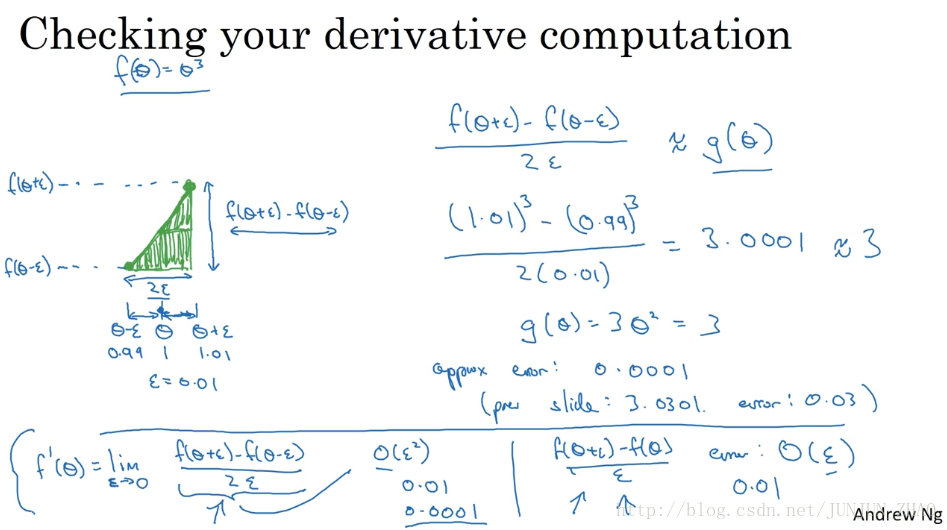
So lets take the function f and replot it here, and remember this is $f(θ)$ equals $θ$ cubed, and let’s again start off some value of theta, let’s say theta equals 1. Now instead of just nudging theta to the right to get theta plus epsilon, we’re going to nudge it to the right and nudge it to the left to get theta minus epsilon, as well as $θ+ε$. So this is 1, this is 1.01, this is 0.99 where, again, epsilon is same as before, it is 0.01. It turns out that rather than taking this little triangle and computing the height over the width, you can get a much better estimate of the gradient if you take this point, f of theta minus epsilon and this point,and you instead compute the height over width of this bigger triangle.So for technical reasons which I won’t go into, the height over width of this bigger green triangle gives you a much better approximation to the derivative at theta.

我们先画出函数 $f$，标记为$f(θ)$ $f(θ)=θ^3$，先看下$θ$的值 假设 $θ=1$，不增大$θ$的值 而是在$θ$右侧，设置一个$θ+ε$，在$θ$左侧 设置$θ-ε$，因此 $θ=1$ $θ+ε=1.01$ $θ-ε=0.99$，跟以前一样$ε$ 的值为 0.01， 看下这个小三角形，计算高和宽的比值 就是更准确的坡度预估，选择$f$函数在$θ-ε$上的这个点，用这个较大三角形的高比上宽，技术上的原因我就不详细解释了，较大三角形的高宽比值更接近于$θ$的导数。

And you saw it yourself, taking just this lower triangle in the upper rightis as if you have two triangles, right?This one on the upper right and this one on the lower left. And you’re kind of taking both of them into account, by using this bigger green triangle. So rather than a one sided difference, you’re taking a two sided difference.

把右上角的三角形下移，好像有了两个三角形，右上角有一个 左下角有一个，我们通过这个绿色大三角形同时考虑了这两个小三角形，所以我们得到的不是一个单边公差而是一个双边公差。

So let’s work out the math.This point here is $f(θ+ε)$.This point here is $f(θ-ε)$.So the height of this big green triangle is $f(θ+ε)-f(θ-ε)$ And then the width, this is 1 epsilon, this is 2 epsilon.So the width of this green triangle is $2ε$.So the height of the width is going to be first the height,so that’s $f(θ+ε)-f(θ-ε)$ divided by the width.So that was $2ε$ which we write that down here.And this should hopefully be close to $g(θ)$.So plug in the values, remember $f(θ)$ is theta cubed.So this is theta plus epsilon is 1.01.So I take a cube of that minus 0.99 take a cube of that, divided by 2 times 0.01.Feel free to pause the video and practice this in the calculator. You should get that this is 3.0001. Whereas from the previous slide, we saw that $g(θ)$, this was 3 theta squared, so when theta was 1, this is 3, $g(θ)=3θ^2$so these two values are actually very close to each other. The approximation error is now 0.0001. Whereas on the previous slide, we’ve taken the one sided of difference, just theta and theta plus epsilon, we had gotten 3.0301 and so the approximation error was 0.03, rather than 0.0001.

我们写一下数据算式，这点的值是$f(θ+ε)$，这点的是$f(θ-ε)$，这个三角形的高度是$f(θ+ε)-f(θ-ε)$，这两个宽度都是 $ε$，所以三角形的宽度是 $2ε$，高宽比值为， $f(θ+ε)-f(θ-ε)$ 除以宽度，宽度为 $2ε$ 结果为 $\dfrac{f(θ+ε)-f(θ-ε)}{2ε}$，它的期望值接近 $g(θ)$，传入参数值 $f(θ)=θ^3$，$θ+ε=1.01$，$\dfrac{(1.01)^3-(0.99)^3}{2(0.01)}$，大家可以暂停视频 用计算器算算结果， 结果应该是 3.0001，而前一张幻灯片上面是，当 θ=1 时 $g(θ)=3$，所以这两个 $g(θ)$ 值非常接近，逼近误差为 0.0001，前一张幻灯片，我们只考虑了单边公差 即从$θ$到$θ+ε$之间的误差，$g(θ)$的值为 3.0301，逼近误差是 0.03 不是 0.0001。

So with this two sided difference way of approximating the derivative you find that this is extremely close to 3. And so this gives you a much greater confidence that $g(θ)$ is probably a correct implementation of the derivative of f.When you use this method for gradient checking and back propagation, this turns out to run twice as slow as you were to use a one-sided difference. It turns out that, in practice, I think it’s worth it to use this other method,because it’s just much more accurate.The little bit of optional theory for those of you that are a little bit more familiar of Calculus,it turns out that, and it’s okay if you don’t get what I’m about to say here.But it turns out that the formal definition of a derivative is for very small values of epsilonis $\dfrac{f(θ+ε)-f(θ-ε)}{2ε}$.And the formal definition of derivative is in the limits of exactlythat formula on the right, as epsilon goes as 0.And the definition of unlimited is something that you learned if you took a Calculus class,but I won’t go into that here.And it turns out that for a non zero value of epsilon,you can show that the error of this approximation is on the order of epsilon squared,and remember epsilon is a very small number.So if epsilon is 0.01, which it is here,then epsilon squared is 0.0001.The big O notation means the error is actually some constant times this, but this is actually exactly our approximation error. So the big O constant happens to be 1.

所以使用双边误差的方法更逼近导数，其结果接近于 3，现在我们更加确信，$g(θ)$可能是一个$f$导数的正确实现，在梯度检验和反向传播中使用该方法时，最终 它与运行两次单边公差的速度一样，实际上 我认为这种方法还是非常值得使用的，因为它的结果更准确，这是一些你可能比较熟悉的微积分的理论，如果你不太明白我讲的这些理论也没关系，导数的官方定义是针对值很小的 $ε$， $\dfrac{f(θ+ε)-f(θ-ε)}{2ε}$，导数的官方定义是右边公式的极限，$ε$趋近于 0，如果你上过微积分课 应该学过无穷尽的定义，我就不在这里讲了，对于一个非零的$ε$，它的逼近误差可以写成 $О(ε^2)$，ε 值非常小，如果 $ε=0.01$， $ε^2$=0.0001，大写符号 O 的含义是指逼近误差其实是一些常量乘以 $ε^2$，但它的确是很准确的逼近误差，所以大写O的常量有时是1。

Whereas in contrast, if we were to use this formula, the other one,then the error is on the order of epsilon.And again, when epsilon is a number less than 1, then epsilon is actuallymuch bigger than epsilon squared, which is why this formula here is actuallymuch less accurate approximation than this formula on the left;which is why when doing gradient checking,we rather use this two-sided difference when you compute $f(θ+ε)-f(θ-ε)$ and then divide by 2ε,rather than just one sided difference which is less accurate. If you didn’t understand my last two comments, all of these things are on here, don’t worry about it. That’s really more for those of you that are a bit more familiar with Calculus, and with numerical approximations.But the takeaway is that this two-sided difference formula is much more accurate.And so that’s what we’re gonna use when we do gradient checking in the next video. So you’ve seen how by taking a two sided difference, you can numerically verify whether or not a function g, $g(θ)$ that someone else gives youis a correct implementation of the derivative of a function f. Let’s now see how we can use this to verify whether or not your back propagation implementation is correct oryou know, there might be a bug in there that you need to go in and tease out.

然而 如果我们用另外一个公式，逼近误差就是$О(ε)$，当$ε$小于 1 时 实际上$ε$比 $ε^2$大很多，所以这个公式，近似值远没有左边公式的准确，所以在执行梯度检验时，我们使用双边误差 即 $\dfrac{f(θ+ε)-f(θ-ε)}{2ε}$ ，而不使用单边公差 因为它不够准确，如果你不理解上面两条结论 所有公式都在这儿，不用担心，如果你对微积分和数值逼近有所了解，这些信息已经足够多了，重点是要记住双边误差公式的结果更准确，下节课我们做梯度检验时就会用到这个方法，今天我们讲了如何使用双边误差，来判断别人给你的函数$g(θ)$，是否正确实现了函数$f$的偏导，现在我们可以使用这个方法来检验，反向传播是否得以正确实施，如果不正确它可能有 bug 需要你来解决。

---

重点总结：

梯度的数值逼近

使用双边误差的方法去逼近导数：

由图可以看出，双边误差逼近的误差是0.0001，先比单边逼近的误差0.03，其精度要高了很多。

涉及的公式：

• 双边导数：

$f'(\theta) = \lim\limits_{\varepsilon \to 0}=\dfrac{f(\theta+\varepsilon)-f(\theta-\varepsilon)}{2\varepsilon}$

误差：$O(\varepsilon^{2})$

• 单边导数：

$f'(\theta) = \lim\limits_{\varepsilon \to 0}=\dfrac{f(\theta+\varepsilon)-f(\theta)}{\varepsilon}$

误差：$O(\varepsilon)$

参考文献：

[1]. 大树先生.吴恩达Coursera深度学习课程 DeepLearning.ai 提炼笔记（2-1）– 深度学习的实践方面

---

PS: 欢迎扫码关注公众号：「SelfImprovementLab」！专注「深度学习」，「机器学习」，「人工智能」。以及 「早起」，「阅读」，「运动」，「英语 」「其他」不定期建群 打卡互助活动。