


1.梯度下降的方式
| 区别 | 梯度下降 | 随机梯度下降(SGD) |
|---|---|---|
| 特点 | 一大块数据一起操作 | 小块数据分开操作 |
| 性能(越高越好) | 低 | 高 |
| 时间复杂度(越低越好) | 低 | 高 |
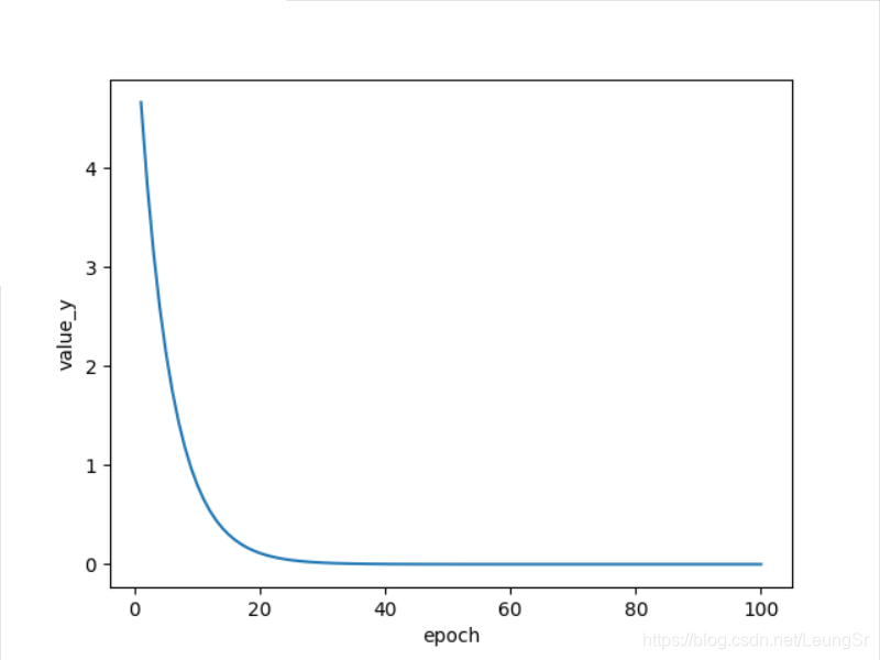
2.朴素梯度下降
# -*- coding:utf-8 -8-
"""
Author: Leung
Date: 2021--08--01
"""
import matplotlib.pyplot as plt
import numpy as np

x_data = [1.0, 2.0, 3.0]
y_data = [2.0, 4.0, 6.0]

w = 1  # 初始化
a = 0.01  # 学习速率


def forward(x):
    return w * x


def cost(xs, ys):
    cost_sum = 0
    assert (len(xs) == len(ys));  # 确定长度相等

    for x_val, y_val in zip(xs, ys):
        y_pred = forward(x_val)
        cost_sum += (y_pred - y_val) * (y_pred - y_val)
    return cost_sum / len(ys)


def back_prog(xs, ys):
    sum_grad = 0

    assert (len(xs) == len(ys))

    for x_val, y_val in zip(xs, ys):
        y_pred = forward(x_val)
        sum_grad += 2 * x_val * (y_pred - y_val)

    delta_w = a * sum_grad / len(ys)

    return delta_w


print("Gradient decent begins...")

cost_vector = []
w_vector = []

for epoch in range(100):
    w_vector.append(w)

    # 计算此时的损失函数
    cost_val = cost(x_data, y_data)
    cost_vector.append(cost_val)

    # 更新w
    delta_w = back_prog(x_data, y_data)
    w = w - delta_w


    print("\t 第", epoch, "次迭代 ", " cost_val = ", cost_val);

x_ax = np.arange(1,101)
# print(x_ax[0])

plt.plot(x_ax, cost_vector)
plt.xlabel("epoch")
plt.ylabel('value_y')
plt.show()

print("the final w: ",w_vector[len(w_vector)-1])
运行结果
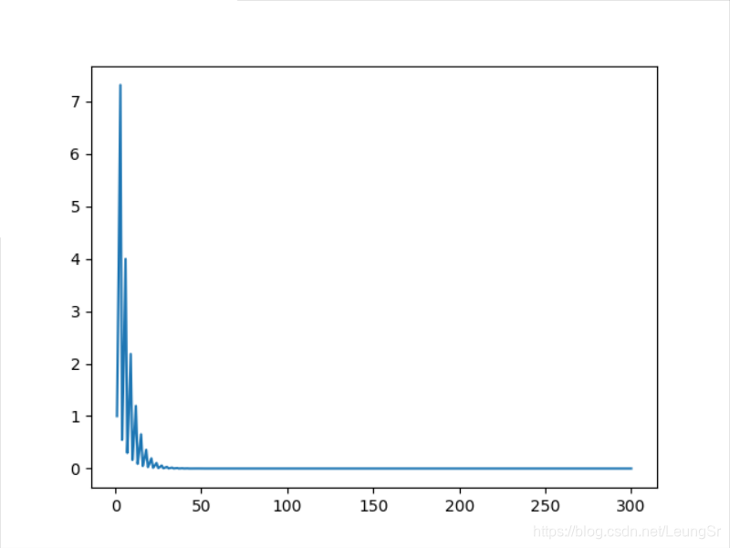
3.随机梯度下降(SGD)
随机梯度下降(Stochastic Gradient Decent)可以在下降的过程中随机地加入一些白噪声,使得我们的在遇到鞍点的情况下仍然能够继续迭代前进(鞍点处的梯度为零,可以类比于 y = x 3 , x = 0 y=x^3,x=0 y=x3,x=0处的导数)
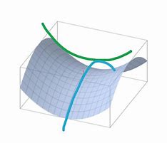
上图为鞍点示意图
# -*- coding:utf-8 -8-
"""
Author: Leung
Date: 2021--08--01
"""

import numpy as np
import matplotlib.pyplot as plt

x_data = [1.0, 2.0, 3.0]
y_data = [2.0, 4.0, 6.0]

w = 1  # 初始化
a = 0.01  # 学习速率


def forward(x):
    return w * x

def loss(xs, ys):
    y_pred = forward(xs)
    return (y_pred - ys) * (y_pred - ys)

def grad(xs, ys):
    y_pred = forward(xs)
    return 2 * xs * (y_pred - ys)

loss_vector =[]

for loop in range(100):
    for x_val,y_val in zip(x_data,y_data):
        loss_vector.append(loss(x_val,y_val))

        w = w-a*grad(x_val,y_val)


x_vector = np.arange(1,301)
plt.plot(x_vector,loss_vector)
plt.show()
运行结果
写在最后
本文章为《PyTorch深度学习实践》完结合集课程对应的一些课后习题解答,仅为各位同志学习参考之用
各位看官,都看到这里了,麻烦动动手指头给博主来个点赞8,您的支持作者最大的创作动力哟! <(^-^)>
才疏学浅,若有纰漏,恳请斧正
本文章仅用于各位同志作为学习交流之用,不作任何商业用途,若涉及版权问题请速与作者联系,望悉知


 296
296


 被折叠的 条评论
为什么被折叠?
被折叠的 条评论
为什么被折叠?
 到【灌水乐园】发言


