俄罗斯酒精消费数据分析（2017-2023）

一、项目背景与数据概况

1.研究背景

俄罗斯作为全球酒精消费大国，其人均酒精消费长期位居世界前五。世界卫生组织发布报告称,五分之一的俄罗斯男性死亡者是因为过量饮酒而毙命的。近年来政府虽推出限酒政策，但消费模式受地域文化、经济结构多重因素影响。

2.数据来源

https://www.kaggle.com/datasets/scibearia/consumption-of-alcohol-in-russia-2017-2023

此数据集显示了 2017 年至 2023 年按地区划分的酒精饮料（伏特加、啤酒、葡萄酒、起泡酒、白兰地和苹果酒）人均消费量的统计数据，覆盖俄罗斯全部85个联邦主体。

3.分析维度

7大类酒品消费量+纯酒精总量，覆盖时间趋势、地区差异、消费模式聚类和未来预测等。

4.数据说明

数据时间范围： 2017年-2023年
数据记录数：595行
字段数：10个
区域覆盖：包含85个地区，覆盖俄罗斯全部联邦主体

字段	说明
Year	年份（2017-2023）
Region	地区名称
Wine	每年人均葡萄酒消费量（升）
Beer	每年人均啤酒消费量（升）
Vodka	每年人均伏特加消费量（升）
Sparkling wine	每年人均起泡酒消费量（升）
Brandy	每年人均白兰地消费量（升）
Cider	每年人均苹果酒消费量（升）
Liqueurs	每年人均利口酒消费量（升）
Total alcohol consumption (in liters of pure alcohol per capita)	每年人均纯酒精总消费量（升）

二、环境准备

1.导入相关库

# 导入库
import pandas as pd
import numpy as np
import matplotlib.pyplot as plt
import seaborn as sns
from sklearn.cluster import KMeans
from sklearn.preprocessing import StandardScaler
from sklearn.ensemble import RandomForestRegressor
from sklearn.metrics import mean_squared_error, silhouette_score
from sklearn.decomposition import PCA
from statsmodels.tsa.arima.model import ARIMA
from statsmodels.tsa.holtwinters import ExponentialSmoothing
from statsmodels.tsa.stattools import adfuller
from scipy.stats import f_oneway, pearsonr
from pmdarima import auto_arima
from matplotlib.patches import Ellipse
from scipy.stats import chi2

2.全局样式设置

# 全局样式设置
plt.rcParams['font.sans-serif'] = ['SimHei']  # 中文字体
plt.rcParams['axes.unicode_minus'] = False  # 负号显示
sns.set_style("whitegrid", {'grid.linestyle': '--'})  # 统一网格样式
sns.set_theme(font='SimHei') # 设置字体
sns.set_context("notebook", font_scale=1.1)  # 设置字体大小
COLOR_PALETTE = sns.color_palette("husl", 8)  # 统一颜色主题

3. 加载数据

修改为对应路径

df = pd.read_csv('Consumption of alcoholic beverages in Russia 2017-2023.csv')

查看数据

df

三、数据预处理与质量检查

1.数据质量验证

重复值和缺失值会干扰数据的准确性，处理缺失值、重复值及异常值是至关重要的步骤，这些操作直接影响到数据分析结果的准确性和可靠性。

print("缺失值统计:\n", df.isnull().sum())
print("重复值数量:", df.duplicated().sum())

这里数据还是比较规范的，没有缺失值和重复值。
如果有缺失值和重复值的话，对其进行填补或者删除等操作。

2.字段重命名

由于 Total alcohol consumption (in liters of pure alcohol per capita) 字段过长，不利于使用的同时影响美观，故重命名为 Pure Alcohol

df = df.rename(columns={"Total alcohol consumption (in liters of pure alcohol per capita)": "Pure Alcohol"})

3.描述性统计

print(df.describe().round(2))

潜在问题：
存在最小值0：数据记录缺失或实际零消费情况（可能性低未查到相关情况）

1. 啤酒为绝对主导品类
   统计数据显示，啤酒的年人均消费量均值为46.46升，远超其他酒类。这与俄罗斯深厚的啤酒文化背景相关，啤酒作为日常饮品和社交媒介，消费场景广泛。
   啤酒消费量的标准差较大（17.25），表明不同地区消费水平差异显著。
2. 伏特加消费趋于稳定
   伏特加的年均消费量为5.56升（标准差2.66），与俄罗斯传统烈酒文化形成一定反差。
   可能与近年来消费者健康意识增强有关，部分转向低酒精或无酒精啤酒。
3. 葡萄酒消费呈小众化
   葡萄酒人均消费量仅3.35升，显著低于啤酒。
   标准差1.64，区域差异小，可能因为消费更集中于高收入或特定文化群体。

四、探索性分析

1. 各酒类年度趋势分析

由于啤酒的值远高于其他酒类，导致其他酒类变化趋势不明显，为了不影响其他酒类趋势分析，选择用双y轴。

#各酒类年度趋势（双Y轴）
yearly_mean = df.groupby('Year').mean(numeric_only=True)

fig, ax = plt.subplots(figsize=(10,6))
yearly_mean[['Wine', 'Vodka', 'Sparkling wine', 'Brandy', 'Сider','Liqueurs']].plot(
    ax=ax, alpha=0.8, color=COLOR_PALETTE[:6], linewidth=2.5,legend=False
)
ax.set_ylabel('其他酒类（升）', color=COLOR_PALETTE[0])
ax.tick_params(axis='y', labelcolor=COLOR_PALETTE[0])

ax2 = ax.twinx()
yearly_mean['Beer'].plot(
    ax=ax2, style='--', color=COLOR_PALETTE[6], linewidth=2.5, 
)
ax2.set_ylabel('啤酒（升）', color=COLOR_PALETTE[6])
ax2.tick_params(axis='y', labelcolor=COLOR_PALETTE[6])
plt.title('各酒类年度消费趋势（2017-2023）', pad=20)
fig.legend(loc="upper left", bbox_to_anchor=(0.15,0.85))
plt.show()

• 啤酒：2020年达峰值，后呈下降趋势，2022年后回温。
  但波动幅度小，受外部影响有限
• 其他酒类：总体幅度缓慢上升，但波动较小

可能原因：
2020年啤酒消费量激增受疫情影响，居家隔离促使家庭储备量上升。2022年后的下降受乌克兰冲突导致的供应链中断影响。

2.纯酒精总消费量趋势与年增长率

# 总消费量趋势与年增长率
total_alcohol = df.groupby('Year')['Pure Alcohol'].mean()
growth_rate = total_alcohol.pct_change() * 100

fig, ax1 = plt.subplots(figsize=(10,6))
ax1.plot(total_alcohol.index, total_alcohol.values, 
         marker='o', color=COLOR_PALETTE[0], linewidth=2.5, label='总消费量')
ax1.set_ylabel('升（纯酒精）', color=COLOR_PALETTE[0])
ax1.tick_params(axis='y', labelcolor=COLOR_PALETTE[0])

# 添加折线图数值标签（使用annotate）
for x, y in zip(total_alcohol.index, total_alcohol.values):
    ax1.annotate(f'{y:.1f}', 
                 (x, y),
                 textcoords="offset points",
                 xytext=(0, 10),
                 ha='center',
                 color=COLOR_PALETTE[0])

ax2 = ax1.twinx()
bars = ax2.bar(growth_rate.index, growth_rate.values, 
               color=COLOR_PALETTE[1], alpha=0.3, width=0.7, label='年增长率')
ax2.axhline(0, color='gray', linestyle='--')
ax2.set_ylabel('增长率 (%)', color=COLOR_PALETTE[1])
ax2.tick_params(axis='y', labelcolor=COLOR_PALETTE[1])

# 修正柱状图标签（改用annotate）
for bar in bars:
    height = bar.get_height()
    x_center = bar.get_x() + bar.get_width()/2  # 计算柱子中心坐标
    
    if height >= 0:
        va = 'bottom'
        offset = 3   # 正数向上偏移3点
    else:
        va = 'top'
        offset = -3  # 负数向下偏移3点
    
    ax2.annotate(f'{height:.1f}%', 
                 xy=(x_center, height),    # 锚点位置（柱子顶部中心）
                 xytext=(0, offset),       # 像素偏移量
                 textcoords='offset points',  # 使用相对偏移坐标
                 ha='center',
                 va=va,
                 color=COLOR_PALETTE[1],
                 fontsize=9,
                 rotation=90)

plt.title('总酒精消费量趋势与年增长率', pad=20)
fig.legend(loc="upper left", bbox_to_anchor=(0.15,0.85))
plt.show()

总酒精消费量持续增长，年均增长2.87%,但增速不稳定。
2019年负增长，呈现"V"型复苏。

可能的原因：
2019年某些酒类价格上调，导致消费减少。
2020受疫情影响，酒类消费增速放缓.

3. 地区消费差异（2023）

#地区消费差异（2023年）
latest_data = df[df['Year'] == 2023].sort_values(
    'Pure Alcohol', 
    ascending=False
).head(10)
# 定义10色渐变色板
COLOR_PALETTE = sns.color_palette("viridis", n_colors=10)[::-1]
plt.figure(figsize=(10,6))
sns.barplot(data=latest_data, 
           x='Pure Alcohol',
           y='Region',
            hue='Region',
           palette=COLOR_PALETTE)
plt.title('2023年地区酒精消费量TOP10', pad=15)
plt.xlabel('人均纯酒精消费量（升）')
plt.ylabel('')
plt.show()

1. 卡累利阿共和国（Republic of Karelia）
   位于北极圈附近，西北边境，与芬兰接壤
2. 萨哈林州（Sakhalin Oblast）
   俄罗斯远东地区唯一出产石油和天然气的地区
3. 科米共和国（Komi Republic）
   位于北极圈附近，自然资源丰富，主要包括石油、天然气、木材、渔业等等
4. 涅涅茨自治区（Nenets Autonomous Okrug）​
   位于北极圈附近，天然气和石油资源丰富
5. 摩尔曼斯克州（Murmansk Oblast）​
   大部分位于北极圈内

共性：

1. 多个地区位于北极圈或近北极地带，气温低，酒精能御寒
2. 多个地区油气、矿产资源丰富，工人多，消费群体多
3. 多个地区位于边境，跨境酒精通道

4. 酒类结构对比

#酒类结构分析
fig, (ax1, ax2) = plt.subplots(1, 2, figsize=(16, 6))
alcohol_types = ['Wine', 'Beer', 'Vodka', 'Sparkling wine', 'Brandy', 'Сider','Liqueurs']
# 各酒类消费量占比（2017年）
past_2017_data = df[df['Year'] == 2023]
past_2017_data[alcohol_types].sum().plot(  
    kind='pie',
    autopct='%1.1f%%',
    title='2017年酒类消费量结构',
    ax=ax1
)
ax2.set_ylabel('')

# 各酒类消费量占比（2023年）
latest_data[alcohol_types].sum().plot(
    kind='pie', autopct='%1.1f%%', title='2023年酒类消费量结构',ax=ax2)
plt.ylabel('')
# 调整布局并展示
plt.tight_layout()
plt.show()

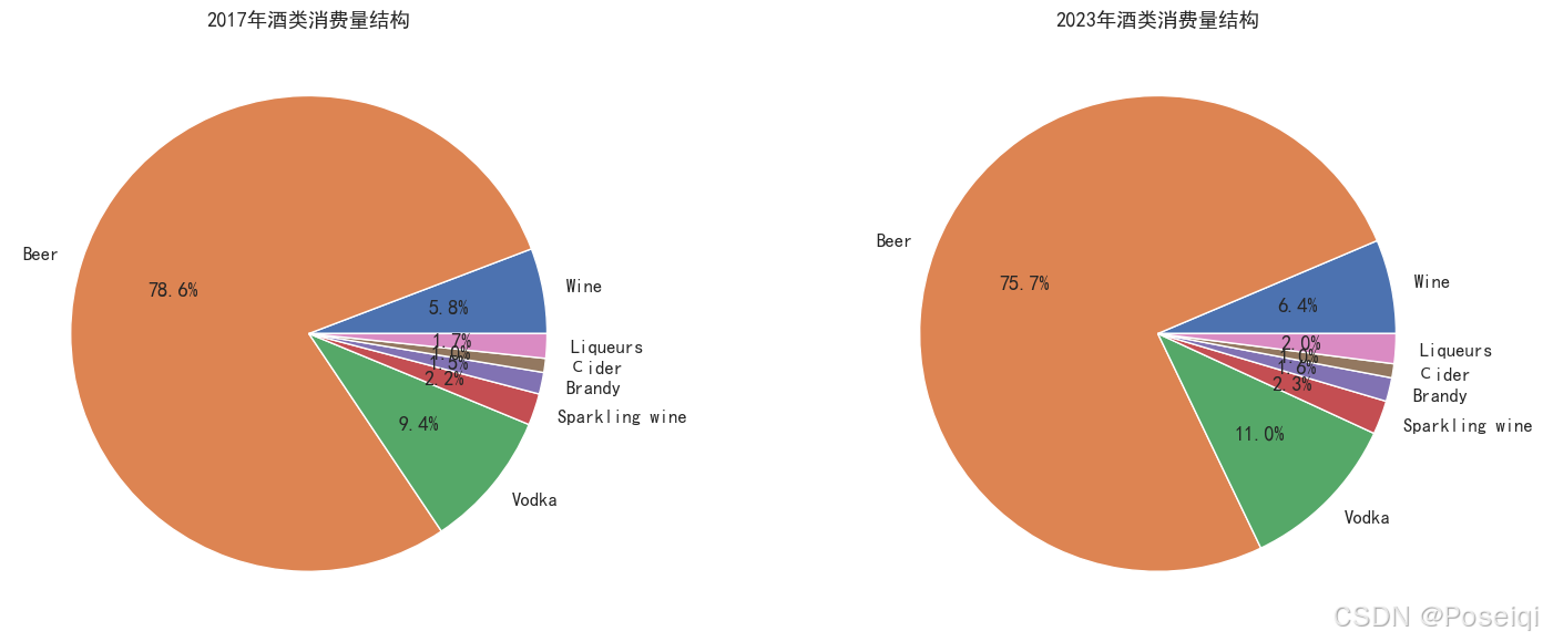
酒类	2017年占比	2023年占比	变化幅度
啤酒	78.6%	75.7%	▼2.9%
伏特加	9.4%	11.0%	▲1.6%
起泡酒	2.2%	2.3%	▲0.1%
白兰地	1.5%	1.6%	▲0.1%
苹果酒	1.0%	1.0%	0
利口酒	1.7%	2.0%	▲0.3%
葡萄酒	5.8%	6.4%	▲0.6%

啤酒地位稳居第一，但有所下降，消费多元化。
伏特加增幅变大，烈酒呈现复苏趋势。

五、聚类分析

肘部法则是最常用的选择K值的方法之一。它通过计算不同K值下的SSE（误差平方和），寻找SSE随着K值的增加而显著减少的拐点。拐点位置通常被认为是最佳的K值，因为在该点之后，SSE的下降幅度会变小。
轮廓系数可以衡量聚类结果的好坏，值的范围在 -1 到 1 之间。值越接近1，说明样本点被良好地聚类；值越接近-1，说明样本点可能被错误聚类。通过计算不同K值下的平均轮廓系数，选择最大轮廓系数对应的K值作为最佳K值。

# 按地区聚合所有年份数据（使用均值）
region_grouped = df.groupby('Region')[['Wine', 'Beer', 'Vodka', 'Sparkling wine', 
                                     'Brandy', 'Сider','Liqueurs','Pure Alcohol']].mean().reset_index()

# 数据标准化
features = region_grouped[['Wine', 'Beer', 'Vodka', 'Sparkling wine', 'Brandy', 'Сider','Liqueurs','Pure Alcohol']]
scaler = StandardScaler()
scaled_features = scaler.fit_transform(features)

# 确定最佳聚类数
fig, (ax1, ax2) = plt.subplots(1,2,figsize=(12,5))

# 肘部法则
sse = []
for k in range(1, 6):
    kmeans = KMeans(n_clusters=k, random_state=42, n_init=10)
    kmeans.fit(scaled_features)
    sse.append(kmeans.inertia_)
ax1.plot(range(1,6), sse, marker='o', color=COLOR_PALETTE[0])
ax1.set_title('肘部法则')
ax1.set_xlabel('聚类数')
ax1.set_ylabel('SSE')

# 轮廓系数
sil_scores = []
for k in range(2, 6):  
    kmeans = KMeans(n_clusters=k, random_state=42, n_init=10)
    labels = kmeans.fit_predict(scaled_features)
    sil_scores.append(silhouette_score(scaled_features, labels))
ax2.plot(range(2,6), sil_scores, marker='o', color=COLOR_PALETTE[1])
ax2.set_title('轮廓系数')
ax2.set_xlabel('聚类数')
plt.tight_layout()
plt.show()

• 肘部法则显示k=2时SSE下降趋缓
• 轮廓系数在k=3时达峰值
• ​最终选择3个消费群体

# 执行聚类（选择k=3）
kmeans = KMeans(n_clusters=3, random_state=42, n_init=10)
region_grouped['Cluster'] = kmeans.fit_predict(scaled_features)

# 聚类可视化
fig = plt.figure(figsize=(15,5))

# 雷达图
ax1 = fig.add_subplot(131, polar=True)
cluster_centers = scaler.inverse_transform(kmeans.cluster_centers_)
angles = np.linspace(0, 2*np.pi, len(features.columns), endpoint=False).tolist()
angles += angles[:1]

for i in range(3):
    values = cluster_centers[i].tolist() + [cluster_centers[i][0]]
    ax1.plot(angles, values, linewidth=2, 
            label=f'Cluster {i}', color=COLOR_PALETTE[i])
    ax1.fill(angles, values, alpha=0.1)
ax1.set_xticks(angles[:-1])
ax1.set_xticklabels(features.columns)
plt.title('聚类特征雷达图', pad=20)

# PCA降维
pca = PCA(n_components=2)
region_grouped[['PCA1','PCA2']] = pca.fit_transform(scaled_features)
ax2 = fig.add_subplot(132)
sns.scatterplot(data=region_grouped, x='PCA1', y='PCA2', hue='Cluster', 
               palette=COLOR_PALETTE[:3], s=80)
plt.title(f'PCA降维分布（累计解释方差：{pca.explained_variance_ratio_.sum():.1%}）')

# 在PCA子图(ax2)中添加置信椭圆
for cluster in range(3):
    # 提取当前簇的PCA数据
    cluster_data = df[df['Cluster'] == cluster][['PCA1', 'PCA2']]
    
    # 计算均值和协方差矩阵
    mean = cluster_data.mean().values
    cov = cluster_data.cov().values
    
    # 计算椭圆参数（95%置信区间）
    lambda_, v = np.linalg.eigh(cov)  # 特征值分解
    angle = np.degrees(np.arctan2(v[0][1], v[0][0]))  # 椭圆旋转角度
    width = 2 * np.sqrt(chi2.ppf(0.95, df=2) * lambda_[0])  # 主轴长度
    height = 2 * np.sqrt(chi2.ppf(0.95, df=2) * lambda_[1])  # 副轴长度
    
    # 绘制椭圆
    ellipse = Ellipse(xy=mean, width=width, height=height, angle=angle,
                      edgecolor=COLOR_PALETTE[cluster], fc='none', 
                      linestyle='--', linewidth=1.5, alpha=0.8)
    ax2.add_patch(ellipse)
    
# 热力图
ax3 = fig.add_subplot(133)
cluster_mean = region_grouped.groupby('Cluster')[features.columns].mean()
sns.heatmap(cluster_mean.T, cmap='Blues', annot=True, fmt=".1f")
plt.title('各聚类平均消费量')
plt.tight_layout()
plt.show()

# 查看各聚类对应的地区列表
for cluster_num in range(3):
    Region = region_grouped[region_grouped['Cluster'] == cluster_num]['Region'].tolist()
    print(f"====== 聚类 {cluster_num} 包含 {len(Region)} 个地区 ======")
    print(Region)
    print("\n")

====== 聚类 0 包含 9 个地区 ======
[‘Chechen Republic’, ‘Kabardino-Balkar Republic’, ‘Karachay-Cherkess Republic’, ‘Republic of Dagestan’, ‘Republic of Ingushetia’, ‘Republic of Kalmykia’, ‘Republic of North Ossetia-Alania’, ‘Stavropol Krai’, ‘Tuva Republic’]

====== 聚类 1 包含 41 个地区 ======
[‘Altai Krai’, ‘Altai Republic’, ‘Astrakhan Oblast’, ‘Belgorod Oblast’, ‘Bryansk Oblast’, ‘Chelyabinsk Oblast’, ‘Chuvash Republic’, ‘Irkutsk Oblast’, ‘Ivanovo Oblast’, ‘Kemerovo Oblast’, ‘Krasnodar Krai’, ‘Krasnoyarsk Krai’, ‘Kurgan Oblast’, ‘Kursk Oblast’, ‘Lipetsk Oblast’, ‘Mari El Republic’, ‘Novosibirsk Oblast’, ‘Omsk Oblast’, ‘Orenburg Oblast’, ‘Oryol Oblast’, ‘Penza Oblast’, ‘Perm Krai’, ‘Republic of Adygea’, ‘Republic of Bashkortostan’, ‘Republic of Buryatia’, ‘Republic of Khakassia’,‘Republic of Mordovia’, ‘Republic of Tatarstan’, ‘Rostov Oblast’,‘Ryazan Oblast’, ‘Sakha (Yakutia) Republic’, ‘Samara Oblast’, ‘Saratov Oblast’, ‘Tambov Oblast’, ‘Tomsk Oblast’, ‘Tula Oblast’, ‘Tyumen Oblast’, ‘Ulyanovsk Oblast’, ‘Volgograd Oblast’, ‘Voronezh Oblast’, ‘Zabaykalsky Krai’]

====== 聚类 2 包含 35 个地区 ======
[‘Amur Oblast’, ‘Arkhangelsk Oblast’, ‘Chukotka Autonomous Okrug’, ‘Jewish Autonomous Oblast’, ‘Kaliningrad Oblast’, ‘Kaluga Oblast’, ‘Kamchatka Krai’, ‘Khabarovsk Krai’, ‘Khanty–Mansi Autonomous Okrug – Yugra’, ‘Kirov Oblast’, ‘Komi Republic’, ‘Kostroma Oblast’, ‘Leningrad Oblast’, ‘Magadan Oblast’, ‘Moscow’, ‘Moscow Oblast’, ‘Murmansk Oblast’, ‘Nenets AutonomousOkrug’, ‘Nizhny Novgorod Oblast’, ‘Novgorod Oblast’, ‘Primorsky Krai’, ‘Pskov Oblast’, ‘Republic of Crimea’, ‘Republic of Karelia’, ‘Saint Petersburg’, ‘Sakhalin Oblast’, ‘Sevastopol’, ‘Smolensk Oblast’, ‘Sverdlovsk Oblast’, ‘Tver Oblast’, ‘Udmurt Republic’, ‘Vladimir Oblast’, ‘Vologda Oblast’, ‘Yamalo-Nenets Autonomous Okrug’, ‘Yaroslavl Oblast’]

• Cluster 0（低消费组）​：
  所有品类消费量显著低于其他聚类
  集中分布于南部温暖气候区
  伏特加（1.3）和纯酒精（1.5）消费量极低
  典型地区：
  车臣共和国（Chechen Republic）​：人口多为穆斯林
  卡尔梅克共和国（Republic of Kalmykia）​：佛教主体地区
• Cluster 1（中等消费组）​：
  伏特加（4.6）和纯酒精（5.6）消费明显上升
  起泡酒、白兰地等酒类开始出现规模性消费
  典型地区：
  鄂木斯克州（Omsk Oblast）​：工业占GDP比重高
  鞑靼斯坦共和国（Republic of Tatarstan）​：民族融合地区，酒类选择多元化
• Cluster 2（高消费组）​：
  所有品类消费量均为最高值
  覆盖北极圈以及周边寒冷地区
  典型地区：
  莫斯科市（Moscow）：俄罗斯的首都，政治、经济、文化和科技的中心。人口多，经济发达。

总结：
Cluster 0：宗教文化主导的非酒精消费模式
Cluster 1：气候-产业协同的中度消费模式
Cluster 2：经济-地理驱动的高消费模式

俄罗斯酒精消费存在显著的区域分异特征，既反映了历史文化传统的影响，也体现了气候经济条件的现实作用。

六、相关性分析

# 计算相关性矩阵
corr_matrix = df[['Wine', 'Beer','Vodka', 'Sparkling wine', 'Brandy', 'Сider','Liqueurs'] + ['Pure Alcohol']].corr()
sns.heatmap(corr_matrix, annot=True, cmap='coolwarm')
plt.title('相关性矩阵')
plt.show()

强相关性组合（红色区域）

• 葡萄酒 & 白兰地 & 起泡酒：消费场景相似，如节日宴会
• 伏特加&纯酒精：伏特加酒精含量高，减少烈酒销售可能直接降低酒精危害。

弱相关性组合（蓝色区域）​

• 伏特加 & 苹果酒：烈酒与果酒几乎无协同，反映完全不同的消费场景

七、消费趋势预测

模型	优势	局限性
随机森林	考虑特征交互，捕捉非线性关系	依赖滞后特征构建
Holt-Winters	擅长趋势外推	忽略品类间关联

1.准备数据

# 准备全国数据
national_df = df.groupby('Year').agg({
    col: 'mean' for col in features.columns
}).reset_index()
national_df['Year_sq'] = (national_df['Year'] - 2017)**2  # 时间趋势项

2.随机森林预测

# 随机森林预测函数
def rf_forecast():
    # 生成滞后特征
    lags = 3
    for col in features.columns:
        for lag in range(1, lags+1):
            national_df[f'{col}_lag{lag}'] = national_df[col].shift(lag)
    rf_df = national_df.dropna().copy()
    
    forecasts = {}
    evaluation = {}  # 存储评估指标
    
    for target in features.columns:
        X = rf_df[[f'{col}_lag{lag}' for col in features.columns for lag in [1,2,3]] + ['Year_sq']]
        y = rf_df[target]
        
        # 划分训练集（排除最后3年）和测试集（最后3年）
        train_size = len(X) - 3
        X_train, X_test = X.iloc[:train_size], X.iloc[train_size:]
        y_train, y_test = y.iloc[:train_size], y.iloc[train_size:]
        
        # 训练模型并预测测试集
        model = RandomForestRegressor(n_estimators=200, max_depth=3, random_state=42)
        model.fit(X_train, y_train)
        y_pred = model.predict(X_test)
        
        # 计算评估指标
        mae = mean_absolute_error(y_test, y_pred)
        rmse = np.sqrt(mean_squared_error(y_test, y_pred))
        evaluation[target] = {'MAE': mae, 'RMSE': rmse}
        
        # 使用全量数据重新训练模型进行未来预测
        model_full = RandomForestRegressor(n_estimators=200, max_depth=3, random_state=42)
        model_full.fit(X, y)
        
        current = rf_df.iloc[-1][X.columns].to_frame().T
        preds = []
        for _ in range(3):
            pred = model_full.predict(current)[0]
            preds.append(pred)
            new_data = current.copy()
            new_data.iloc[:, :len(features.columns)] = np.roll(
                new_data.iloc[:, :len(features.columns)].values, 
                shift=-1, 
                axis=1
            )
            new_data.iloc[0, 0] = pred
            current = new_data
        
        forecasts[target] = preds
        
    return forecasts, evaluation

rf_results, rf_metrics = rf_forecast()

3.Holt-Winters预测

# Holt-Winters预测函数
def hw_forecast():
    national_ts = national_df.copy()
    national_ts['Year'] = pd.to_datetime(national_ts['Year'], format='%Y')
    national_ts = national_ts.set_index('Year').asfreq('YS').sort_index()
    
    forecasts = {}
    evaluation = {}  # 存储评估指标
    
    for col in features.columns:
        ts_data = national_ts[col]
        
        # 划分训练集（排除最后3年）和测试集（最后3年）
        train = ts_data.iloc[:-3]
        test = ts_data.iloc[-3:]
        
        # 训练模型并预测测试集
        try:
            model_train = ExponentialSmoothing(
                train, trend='add', seasonal=None,
                initialization_method="estimated"
            )
            model_train_fit = model_train.fit()
            forecast_test = model_train_fit.forecast(steps=3)
            
            # 计算评估指标
            mae = mean_absolute_error(test, forecast_test)
            rmse = np.sqrt(mean_squared_error(test, forecast_test))
            evaluation[col] = {'MAE': mae, 'RMSE': rmse}
        except Exception as e:
            print(f"Error in {col}: {str(e)}")
            evaluation[col] = {'MAE': np.nan, 'RMSE': np.nan}
        
        # 使用全量数据重新训练模型
        model_full = ExponentialSmoothing(
            ts_data, trend='add', seasonal=None,
            initialization_method="estimated"
        )
        model_full_fit = model_full.fit()
        forecast = model_full_fit.forecast(steps=3)
        forecasts[col] = forecast.tolist()
        
    return forecasts, evaluation

hw_results, hw_metrics = hw_forecast()

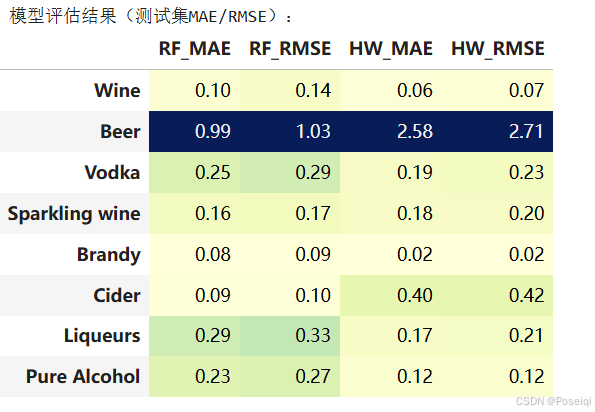
4.可视化对比

• MAE 是预测值与实际值之差的绝对值的平均数。它给出了预测误差的平均大小，但不考虑误差的方向（正或负）。
• 均方根误差（RMSE） 是均方误差（MSE）的平方根。MSE是衡量预测值与实际值之间平方差的平均值，而RMSE则将其量级与原始数据保持一致，便于解释。由于计算了平方差，RMSE对大误差的惩罚更大，适合对误差敏感的场景。

# 创建评估指标对比表格
metrics_df = pd.DataFrame({
    'RF_MAE': [rf_metrics[col]['MAE'] for col in features.columns],
    'RF_RMSE': [rf_metrics[col]['RMSE'] for col in features.columns],
    'HW_MAE': [hw_metrics[col]['MAE'] for col in features.columns],
    'HW_RMSE': [hw_metrics[col]['RMSE'] for col in features.columns]
}, index=features.columns)

# 添加评估结果到可视化
fig, axes = plt.subplots(4, 2, figsize=(18, 22))
for idx, col in enumerate(features.columns):
    ax = axes[idx//2, idx%2]
    
    # 历史数据
    ax.plot(national_df['Year'], national_df[col], 
           marker='o', color=COLOR_PALETTE[0], label='历史数据')
    
    # 预测数据
    years = [2024, 2025, 2026]
    ax.plot(years, rf_results[col], 
           marker='s', linestyle='--', color=COLOR_PALETTE[1], 
           label=f'随机森林 (MAE:{rf_metrics[col]["MAE"]:.2f}, RMSE:{rf_metrics[col]["RMSE"]:.2f})')
    ax.plot(years, hw_results[col], 
           marker='^', linestyle='-.', color=COLOR_PALETTE[2], 
           label=f'Holt-Winters (MAE:{hw_metrics[col]["MAE"]:.2f}, RMSE:{hw_metrics[col]["RMSE"]:.2f})')
    
    ax.set_title(f'{col}消费量预测对比')
    ax.set_ylabel('升（人均）')
    ax.axvline(2023, color='gray', linestyle='--')
    ax.legend()

plt.tight_layout()
plt.show()

# 打印评估结果表格
print("模型评估结果（测试集MAE/RMSE）：")
display(metrics_df.style.format("{:.2f}").background_gradient(axis=0, cmap='YlGnBu'))

# 创建对比表格，将预测列表格式化为字符串
forecast_df = pd.DataFrame({
    '随机森林': [', '.join(f"{x:.2f}" for x in rf_results[col]) for col in features.columns],
    'Holt-Winters': [', '.join(f"{x:.2f}" for x in hw_results[col]) for col in features.columns]
}, index=features.columns)

print("2024-2026年预测结果对比（升/人均）：")
display(forecast_df.style.background_gradient(axis=0, cmap='YlGnBu'))

总结

总体增长：
2017-2023年俄罗斯人均纯酒精消费量年均增长2.87%，但增速受疫情和政策调控影响显著波动（如2020年负增长）。

品类分化：
啤酒占主导地位（2023占比75.7%），但有所下降，消费呈现多元化。
伏特加增幅变大，烈酒呈现复苏趋势。消费存在地域差别，与纯酒精消费高度绑定（r=0.93），反映烈酒仍是酒精摄入的主要载体。

区域分异：

• 高消费集群（Cluster 2）：集中于北极圈及资源型地区，纯酒精消费量达全国均值1.6倍，受气候和经济收入影响。
• 低消费集群（Cluster 0）：消费量仅为全国均值的29%，宗教政策抑制效果显著。

模型预测：

• 未来趋势： 2024-2026年啤酒消费预计年均下降1.5%
• 健康风险： 世界卫生组织编写的一份报告强调指出，2019年有260万人死于饮酒，占死亡总人数的4.7%。饮酒所带来的危害已经成为影响健康，危机群体安全的社会问题。

建议：

1. 提升低度酒类市场份额，增加低酒精和无酒精饮品销售。
2. 加强烈酒消费管控，减少酒精依赖。
3. 构建酒精消费-疾病关联数据库，实时监控高危区域，为医疗资源调度提供依据。