添加行政区域线的气象要素分布图

首先需要下载行政区域线的.shp文件。网络上的常用方法是从GADM网站上下载。

笔者现有行政区域图的.geojson文件，可通过代码直接转化为.shp

代码如下：

import geopandas as gpd
import os
import sys

# 设置 GDAL_DATA 环境变量（路径根据实际安装位置修改）
gdal_data_path = r"D:\app\anaconda\envs\py312\Library\share\gdal"  # 需验证路径是否存在：

if os.path.exists(gdal_data_path):
    os.environ['GDAL_DATA'] = gdal_data_path
else:
    print(f"错误：GDAL_DATA 路径不存在 {gdal_data_path}")
    print("请通过以下方式查找正确路径：")
    print("1. 在Anaconda环境目录中搜索 'header.dxf'")
    print("2. 找到类似 '.../Library/share/gdal' 的目录")
    print("3. 修改代码中 gdal_data_path 变量")
    sys.exit(1)

# ========== 原始转换代码 ==========
# 读取GeoJSON文件
input_path = r"D:\xian.geojson"
gdf = gpd.read_file(input_path)

# 定义输出路径
output_dir = r"D:\xian_1"
output_filename = "xian.shp"
os.makedirs(output_dir, exist_ok=True)

output_path = os.path.join(output_dir, output_filename)

# 修复字段名长度问题
gdf.columns = [col[:10] for col in gdf.columns]  # Shapefile字段名最多10字符

# 保存文件
try:
    gdf.to_file(output_path, encoding='utf-8')
    print(f"文件已保存到：{output_path}")
    print("生成的文件列表：")
    for f in os.listdir(output_dir):
        if f.startswith(output_filename.split(".")[0]):
            print(f" - {f}")
except Exception as e:
    print(f"保存失败：{str(e)}")
    print("可能原因：")
    print("1. 文件正在被其他程序占用")
    print("2. 输出目录没有写入权限")
    print("3. 几何数据存在错误（尝试 gdf = gdf.make_valid()）")

转为.shp文件后可在绘图代码中应用：

import xarray as xr
import matplotlib.pyplot as plt
import cartopy.crs as ccrs
import cartopy.feature as cfeature
from matplotlib.colors import BoundaryNorm
from cartopy.io.shapereader import Reader
from cartopy.feature import ShapelyFeature

plt.rcParams['font.sans-serif'] = ['SimHei']  
plt.rcParams['axes.unicode_minus'] = False   

ds = xr.open_dataset(r"D:\x.nc")

fig = plt.figure(figsize=(12, 8), dpi=300)
ax = fig.add_axes([0.08, 0.1, 0.72, 0.8], projection=ccrs.PlateCarree()) 
proj = ccrs.PlateCarree()

province_path = r"D:\xian.shp"
provinces = ShapelyFeature(
    Reader(province_path).geometries(),
    crs=proj,
    edgecolor='black',
    facecolor='none',
    linewidth=0.3,
    linestyle='-'
)
ax.add_feature(provinces, zorder=2)

scale = '50m'
base_style = {'linewidth': 0.5}

ax.add_feature(cfeature.COASTLINE.with_scale(scale), edgecolor='black', **base_style)
ax.add_feature(cfeature.BORDERS.with_scale(scale), linestyle=':', edgecolor='black', **base_style)
ax.add_feature(cfeature.LAKES.with_scale(scale),
              edgecolor='black', facecolor='lightblue', alpha=0.3, **base_style)
ax.add_feature(cfeature.RIVERS.with_scale(scale), edgecolor='dodgerblue', **base_style)

levels = [0, 0.1, 2, 5, 10, 20, 30, 40, 50, 75, 100]
colors = ['#f0f9e8', '#bae4bc', '#7bccc4', '#43a2ca', '#0868ac', '#084081', '#49006a']
cmap = plt.get_cmap('Blues').from_list('custom', colors, N=len(levels)-1)
norm = BoundaryNorm(levels, ncolors=len(levels)-1)

rain_plot = ax.contourf(
    ds.longitude,
    ds.latitude,
    total_rain,
    levels=levels,
    cmap=cmap,
    norm=norm,
    extend='max',
    transform=proj
)


cbar = plt.colorbar(rain_plot, ax=ax, pad=0.08, aspect=40, ticks=levels)
cbar.set_label('XXXX (mm)', fontsize=6, labelpad=8, rotation=270)
cbar.ax.tick_params(labelsize=6)

ax.add_feature(cfeature.LAND.with_scale(scale), zorder=1, edgecolor='k', facecolor='lightgray', alpha=0.2)

gl = ax.gridlines(
    crs=proj,
    draw_labels=True,
    linewidth=0.3,
    color='gray',
    alpha=0.5,
    linestyle='--'
)
gl.top_labels = False
gl.right_labels = False
gl.xlabel_style = {'size': 6, 'color': 'black'}
gl.ylabel_style = {'size': 6, 'color': 'black'}

ax.set_title('XXXX\n2029年3月11-12日', fontsize=10, pad=8, fontweight='bold')
ax.set_extent([73, 144, 3, 55], crs=proj)

plt.subplots_adjust(left=0.08, right=0.85, top=0.9, bottom=0.1) 

# plt.savefig('rainfall_map_highres.png', bbox_inches='tight', dpi=300)
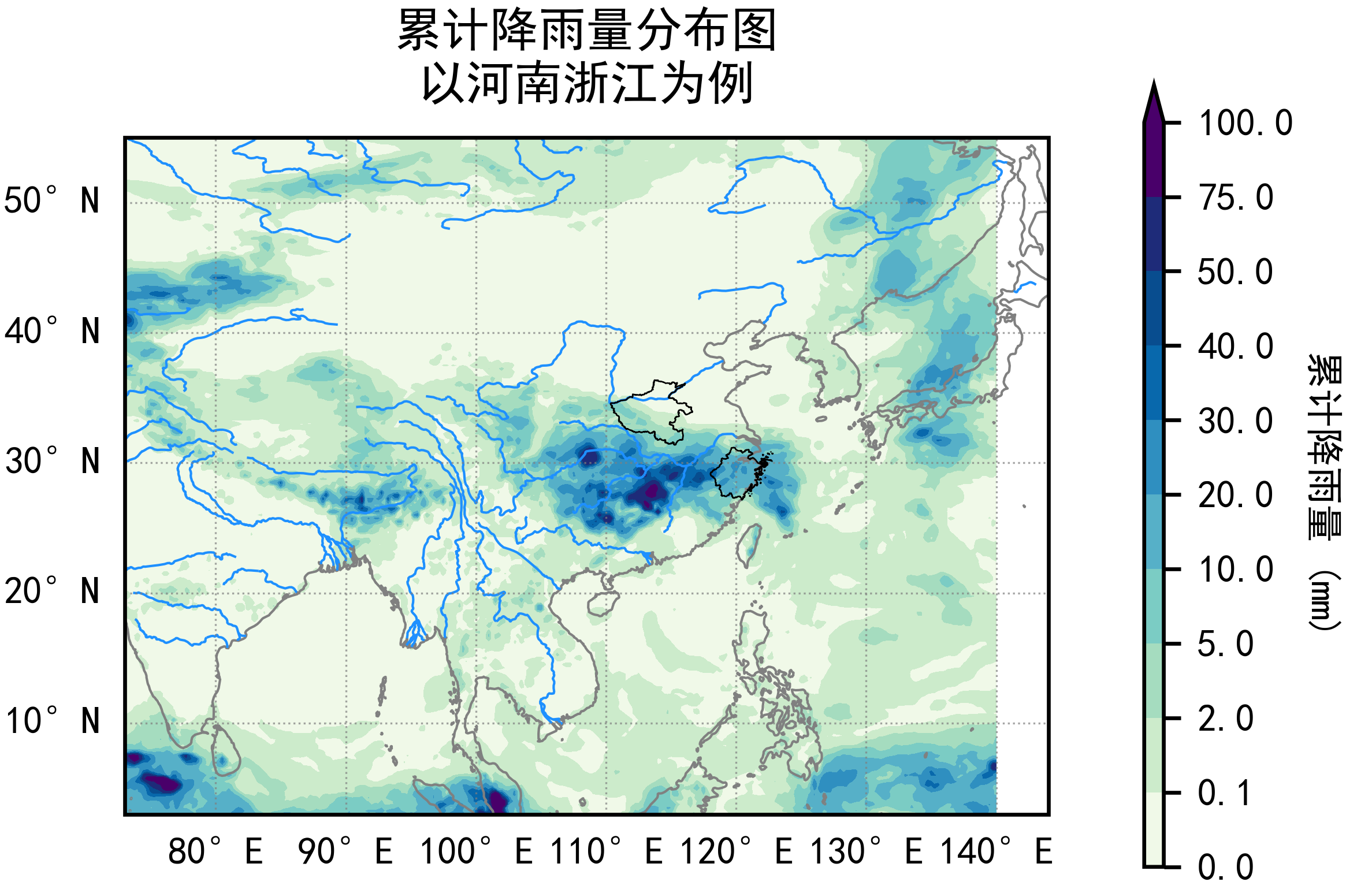
plt.show()

绘制成功后例图如下：