


有关公式、基本理论等大量内容摘自《动手学深度学习》(TF2.0版))
命令式编程和符号式编程是什么?
命令式编程,用直白的话就是:我们写的那种通常写的那种方式,使用编程语句改变程序状态,明确输入变量,并根据程序逻辑逐步运算。
例如如下代码:
import time
import tensorflow as tf
#命令式编程
def add(a, b):
    return a + b

def fancy_func(a, b, c, d):
    e = add(a, b)
    f = add(c, d)
    g = add(e, f)
    return g
begin = time.time()
print(fancy_func(1, 2, 3, 4)) # 10
end = time.time()
#*100方便观察
print("运行时间:",(end-begin)*100)
而符号式编程则是通常在计算流程完全定义好后才被执行。
例如如下代码:
import time
import tensorflow as tf
#符号式编程
def add_str():
    return '''
def add(a, b):
    return a + b
'''

def fancy_func_str():
    return '''
def fancy_func(a, b, c, d):
    e = add(a, b)
    f = add(c, d)
    g = add(e, f)
    return g
'''

def evoke_str():
    return add_str() + fancy_func_str() + '''
print(fancy_func(1, 2, 3, 4))
'''

prog = evoke_str()
print(prog)
#通过compile函数编译完整的计算流程
y = compile(prog, '', 'exec')
begin = time.time()
#运行
exec(y)# 10
end = time.time()
#*100方便观察
print("运行时间:",(end-begin)*100)
命令式编程:写起来很方便,因为就是我们最常写的方式,并且调试很简单,因为可以很方便地进行单步跟踪,获取并分析所有中间变量,或者使用Python的调试工具。但是运行速度慢、浪费空间,其原因就是按照我们写的命令执行,缺少许多系统优化。
符号式编程:更高效、更容易移植,原因是符号式编程可以将程序变成一个与Python无关的格式,该格式类似一个图,可以进行很多优化,并且该格式与可以被奇特语言使用,同时,在编译时系统能够完整地获取整个程序,因此有更多空间优化计算,不仅减少了函数调用,还节省了内存,所以更高效和更容易移植。但是别写符号式编程比较困难,不是很符合人们的编程。
仅仅已上述代码运行时间进行观察(时间均扩大了一百倍,方便观察):
命令式运行时间: 0.0013113021850585938
符号式运行时间: 0.0007867813110351562
可以发现符号式编程比命令式编程更加快速。
- 命令式编程容易理解和调试,命令语句基本没有优化,按原有逻辑执行。
- 符号式编程涉及较多的嵌入和优化,不容易理解和调试,但运行速度有同比提升。
规范说法:

通过上述考虑,我们可以认为:编写时用命令式编程,但是计算机自动转化为符号式编程,然后实际运行的代码是等价的符号式编程是最理想~那么能实现吗?
这就是下面要说的混合式编程~

(官方说法前面说的是背景,后面很多人不理解,其实对于目前不是很理解的人来说,可以这么理解:使用tf.function就是混合式编程,也就是我们说的编写的命令式,执行的却是符号式)
例如几个常见的例子
定义一个Tensorflow
@tf.function
def add(a, b):
    return a+b

add(tf.ones([2, 2]), tf.ones([2, 2]))  #  [[2., 2.], [2., 2.]]
执行上述并求梯度
v = tf.Variable(1.0)
with tf.GradientTape() as tape:
    result = add(v, 1.0)
tape.gradient(result, v)
嵌套定义(在实际使用中,可以直接在顶层定义,会自动对子图进行转换)
@tf.function
def dense_layer(x, w, b):
  return add(tf.matmul(x, w), b)

dense_layer(tf.ones([3, 2]), tf.ones([2, 2]), tf.ones([2]))
tf.function特性:追踪与多态

import time
import tensorflow as tf
@tf.function
def double(a):
  print("Tracing with", a)
  return a + a

print(double(tf.constant(1)))
print()
print(double(tf.constant(1.1)))
print()
print(double(tf.constant("a")))
print()
输出:
Tracing with tf.Tensor(1, shape=(), dtype=int32)
tf.Tensor(2, shape=(), dtype=int32)

Tracing with tf.Tensor(1.1, shape=(), dtype=float32)
tf.Tensor(2.2, shape=(), dtype=float32)

Tracing with tf.Tensor(b'a', shape=(), dtype=string)
tf.Tensor(b'aa', shape=(), dtype=string)
上述代码输出与不添加@tf.function一致,说明实现了追踪功能。

import time
import tensorflow as tf
from numpy.testing import assert_raises
print("获取具体痕迹")
double_strings = double.get_concrete_function(tf.TensorSpec(shape=None, dtype=tf.string))
print("执行跟踪函数")
print(double_strings(tf.constant("a")))
print(double_strings(a=tf.constant("b")))
print("使用具有不兼容类型的具体跟踪将引发错误")
with assert_raises(tf.errors.InvalidArgumentError):
  double_strings(tf.constant(1))

@tf.function(input_signature=(tf.TensorSpec(shape=[None], dtype=tf.int32),))
def next_collatz(x):
  print("Tracing with", x)
  return tf.where(x % 2 == 0, x // 2, 3 * x + 1)

print(next_collatz(tf.constant([1, 2])))
# We specified a 1-D tensor in the input signature, so this should fail.
with assert_raises(ValueError):
  next_collatz(tf.constant([[1, 2], [3, 4]]))
结果:
获取具体痕迹
Tracing with Tensor("a:0", dtype=string)
执行跟踪函数
tf.Tensor(b'aa', shape=(), dtype=string)
tf.Tensor(b'bb', shape=(), dtype=string)
使用具有不兼容类型的具体跟踪将引发错误
Tracing with Tensor("x:0", shape=(None,), dtype=int32)
tf.Tensor([4 1], shape=(2,), dtype=int32)
资料中结果:
Tracing with Tensor("x:0", shape=(None,), dtype=int32)
tf.Tensor([4 1], shape=(2,), dtype=int32)
Caught expected exception
  <class 'ValueError'>:

Traceback (most recent call last):
  File "<ipython-input-3-73d0ca52e838>", line 8, in assert_raises
    yield
  File "<ipython-input-9-9939c82c1507>", line 9, in <module>
    next_collatz(tf.constant([[1, 2], [3, 4]]))
ValueError: Python inputs incompatible with input_signature:
  inputs: (
    tf.Tensor(
[[1 2]
 [3 4]], shape=(2, 2), dtype=int32))
  input_signature: (
    TensorSpec(shape=(None,), dtype=tf.int32, name=None))
(说实话这里不是很懂...,结果也不太一样,大家可以查阅其他资料研究研究~)
tf.function特性:追踪触发的时机

tf.function特性:输入参数的选择 Python or Tensor

![]()
这里我们通过两个代码来进行观察
代码1:
import time
import tensorflow as tf
@tf.function
def train(num_steps):
  print("是否触发")
  print("Tracing with num_steps = {}".format(num_steps))
  #模拟模型训练过程
  for _ in tf.range(num_steps):
    train_one_step()

train(num_steps=10)
train(num_steps=20)

train(num_steps=tf.constant(10))
train(num_steps=tf.constant(20))
结果:
是否触发
Tracing with num_steps = 10
是否触发
Tracing with num_steps = 20
是否触发
Tracing with num_steps = Tensor("num_steps:0", shape=(), dtype=int32)
代码2:
import time
import tensorflow as tf
def train(num_steps):
  print("是否触发")
  print("Tracing with num_steps = {}".format(num_steps))
  #模拟模型训练过程
  for _ in tf.range(num_steps):
    train_one_step()

train(num_steps=10)
train(num_steps=20)

train(num_steps=tf.constant(10))
train(num_steps=tf.constant(20))
结果:
是否触发
Tracing with num_steps = 10
是否触发
Tracing with num_steps = 20
是否触发
Tracing with num_steps = 10
是否触发
Tracing with num_steps = 20
通过上述代码我们可以发现,使用tf.function对于某一函数,输入不同的参数可以减少生成图的触发。
tf.function特性:tf.function 的附带效应
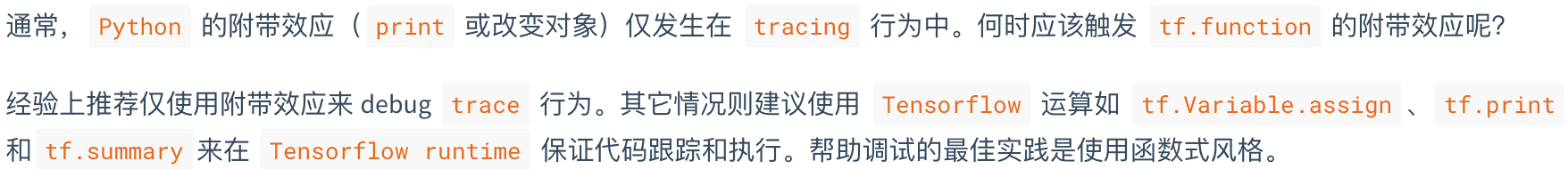
(我个人感觉...这里的意思是:python函数和tf函数在tf.function中的区别~ 可能有理解偏差...)
用个代码来展示下:
@tf.function
def f(x):
  print("Traced with", x)
  tf.print("Executed with", x)

f(1)
f(1)
f(2)
print("---------------")
结果:

(可以发现print是输出的出来的,而且如果图不触发时不会调用,而tf.print更类似一种系统输出,然后即使图不再次生成也可以输出更适合追踪信息)

(综上可知,我们尽量使用前者的tf.function和tf.print方法)
这里提供一个代码,给大家看一下上述后者方式
import time
import tensorflow as tf
external_list = []

def side_effect(x):
  print('Python side effect')
  external_list.append(x)

@tf.function
def f(x):
  tf.py_function(side_effect, inp=[x], Tout=[])

f(1)
f(1)
f(1)
print(len(external_list))
print(external_list)
结果:
Python side effect
Python side effect
Python side effect
3
[<tf.Tensor: id=186, shape=(), dtype=int32, numpy=1>, <tf.Tensor: id=187, shape=(), dtype=int32, numpy=1>, <tf.Tensor: id=188, shape=(), dtype=int32, numpy=1>]
可以看出来,符合上述的描述。
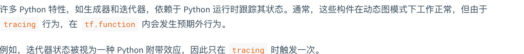
tf.function特性:注意 Python 的状态
代码如下:
import time
import tensorflow as tf
external_var = tf.Variable(0)
@tf.function
def buggy_consume_next(iterator):
  external_var.assign_add(next(iterator))
  tf.print("Value of external_var:", external_var)
  tf.print(iterator)

iterator = iter([0, 1, 2, 3])
buggy_consume_next(iterator)
buggy_consume_next(iterator)
buggy_consume_next(iterator)
结果如下:
Value of external_var: 0
<list_iterator object at 0x7f861fcb2a90>
Value of external_var: 0
<list_iterator object at 0x7f861fcb2a90>
Value of external_var: 0
<list_iterator object at 0x7f861fcb2a90>
(这里我有个疑问...通过上述我们可以发现迭代器方式可以只触发一次,不应该是只生成一个计算图嘛...为什么还是会产生大量计算图,迷糊~)
演示代码:
import time
import tensorflow as tf
#计算图结点数量
def measure_graph_size(f, *args):
  g = f.get_concrete_function(*args).graph
  #print(g)
  print("{}({}) 图中包含 {} 个结点".format(
      f.__name__, ', '.join(map(str, args)), len(g.as_graph_def().node)))
#模拟训练过程
@tf.function
def train(dataset):
  loss = tf.constant(0)
  for x, y in dataset:
    loss += tf.abs(y - x) # Some dummy computation.
  return loss
#生成两个数据集进行测试
small_data = [(1, 1)] * 2
big_data = [(1, 1)] * 10
#数据集直接进行测试
measure_graph_size(train, small_data)
measure_graph_size(train, big_data)
#数据集先转化再测试
measure_graph_size(train, tf.data.Dataset.from_generator(
    lambda: small_data, (tf.int32, tf.int32)))
measure_graph_size(train, tf.data.Dataset.from_generator(
    lambda: big_data, (tf.int32, tf.int32)))
结果:
train([(1, 1), (1, 1)]) 图中包含 8 个结点
train([(1, 1), (1, 1), (1, 1), (1, 1), (1, 1), (1, 1), (1, 1), (1, 1), (1, 1), (1, 1)]) 图中包含 32 个结点
train(<DatasetV1Adapter shapes: (<unknown>, <unknown>), types: (tf.int32, tf.int32)>) 图中包含 5 个结点
train(<DatasetV1Adapter shapes: (<unknown>, <unknown>), types: (tf.int32, tf.int32)>) 图中包含 5 个结点
可以发现,确实有不同,不过具体细节我就不知道了...

tf.function特性:自动控制依赖

tf.function特性:变量

有歧义代码:
import time
import tensorflow as tf
from numpy.testing import assert_raises
@tf.function
def f(x):
  v = tf.Variable(1.0)
  v.assign_add(x)
  return v

with assert_raises(ValueError):
  print(f(1.0))
(结果不太一样~后续再研究吧~)
而无歧义的代码就不会触发相应的行为
无歧义代码:
import time
import tensorflow as tf
v = tf.Variable(1.0)

@tf.function
def f(x):
  return v.assign_add(x)

print(f(1.0))  # 2.0
print(f(2.0))  # 4.0
只要可以证明tf.function中的变量只在函数初次执行时被创建,也是可以通过检查的。
import time
import tensorflow as tf
class C:
  pass

obj = C()
obj.v = None

@tf.function
def g(x):
  if obj.v is None:
    obj.v = tf.Variable(1.0)
  return obj.v.assign_add(x)

print(g(1.0))  # 2.0
print(g(2.0))  # 4.0
AutoGraph

@tf.function
def f(x):
  while tf.reduce_sum(x) > 1:
    tf.print(x)
    x = tf.tanh(x)
  return x

f(tf.random.uniform([5]))
print("---------------")
def f(x):
  while tf.reduce_sum(x) > 1:
    tf.print(x)
    x = tf.tanh(x)
  return x
#输出autograph 生成的代码
print(tf.autograph.to_code(f))
(使用@tf.function修饰的函数无法查看代码,所以又写了个)
结果(2个分别截图了):


AutoGraph:条件分支

代码如下:
import time
import tensorflow as tf
#test_tf_cond 函数用来检查函数中是否使用了 tf.cond
def test_tf_cond(f, *args):
  g = f.get_concrete_function(*args).graph
  if any(node.name == 'cond' for node in g.as_graph_def().node):
    print("{}({}) uses tf.cond.".format(
        f.__name__, ', '.join(map(str, args))))
  else:
    print("{}({}) executes normally.".format(
        f.__name__, ', '.join(map(str, args))))

  print("  result: ",f(*args).numpy())

@tf.function
def dropout(x, training=True):
  if training:
    x = tf.nn.dropout(x, rate=0.5)
  return x
#当参数为 python True 时,正常地执行条件
test_tf_cond(dropout, tf.ones([10], dtype=tf.float32), True)
#但传递一个张量则会使 python if 替换为 tf.cond
test_tf_cond(dropout, tf.ones([10], dtype=tf.float32), tf.constant(True))
结果:
dropout(tf.Tensor([1. 1. 1. 1. 1. 1. 1. 1. 1. 1.], shape=(10,), dtype=float32), True) executes normally.
  result:  [2. 2. 2. 0. 2. 0. 2. 2. 2. 0.]
dropout(tf.Tensor([1. 1. 1. 1. 1. 1. 1. 1. 1. 1.], shape=(10,), dtype=float32), tf.Tensor(True, shape=(), dtype=bool)) uses tf.cond.
  result:  [2. 2. 2. 0. 2. 0. 2. 2. 2. 2.]
AutoGraph 与循环

展示代码如下:
import time
import tensorflow as tf
#实现转化的函数
def test_dynamically_unrolled(f, *args):
  g = f.get_concrete_function(*args).graph
  if any(node.name == 'while' for node in g.as_graph_def().node):
    print("{}({}) uses tf.while_loop.".format(
        f.__name__, ', '.join(map(str, args))))
  elif any(node.name == 'ReduceDataset' for node in g.as_graph_def().node):
    print("{}({}) uses tf.data.Dataset.reduce.".format(
        f.__name__, ', '.join(map(str, args))))
  else:
    print("{}({}) gets unrolled.".format(
        f.__name__, ', '.join(map(str, args))))
#f根据函数名字判断类型
@tf.function
def for_in_range():
  x = 0
  for i in range(5):
    x += i
  return x

test_dynamically_unrolled(for_in_range)
@tf.function
def for_in_tfrange():
  x = tf.constant(0, dtype=tf.int32)
  for i in tf.range(5):
    x += i
  return x

test_dynamically_unrolled(for_in_tfrange)
@tf.function
def for_in_tfdataset():
  x = tf.constant(0, dtype=tf.int64)
  for i in tf.data.Dataset.range(5):
    x += i
  return x

test_dynamically_unrolled(for_in_tfdataset)
@tf.function
def while_py_cond():
  x = 5
  while x > 0:
    x -= 1
  return x

test_dynamically_unrolled(while_py_cond)
@tf.function
def while_tf_cond():
  x = tf.constant(5)
  while x > 0:
    x -= 1
  return x

test_dynamically_unrolled(while_tf_cond)
结果:
for_in_range() gets unrolled.
for_in_tfrange() uses tf.while_loop.
for_in_tfdataset() uses tf.data.Dataset.reduce.
while_py_cond() gets unrolled.
while_tf_cond() uses tf.while_loop.
小结:
上述其实感觉是框架的使用或者说某些优化,单纯学习深度学习可能不太理解,建议学习一下tf2.0这个框架,其实我也很多不太明白的...毕竟从1.4过来的,外加1.x也没学的很明白,仅仅是会使用框架使用模型~
异步计算


示例代码:
a = tf.ones((1, 2))
b = tf.ones((1, 2))
c = a * b + 2
print(c)


import tensorflow as tf
import tensorflow.keras as keras
import os
import subprocess
import time
#定义时钟类
class Benchmark(object):
  def __init__(self, prefix=None):
    self.prefix = prefix + ' ' if prefix else ''

  def __enter__(self):
    self.start = time.time()

  def __exit__(self, *args):
    print('%stime: %.4f sec' % (self.prefix, time.time() - self.start))
with Benchmark('Workloads are queued.'):
  x = tf.random.uniform(shape=(2000, 2000))
  y = tf.keras.backend.sum(tf.transpose(x) * x)

with Benchmark('Workloads are finished.'):
  print('sum =', y)
结果:
Workloads are queued. time: 0.0927 sec
sum = tf.Tensor(999789.06, shape=(), dtype=float32)
Workloads are finished. time: 0.0001 sec
用同步函数让前端等待计算结果

(具体不举例子了~)

使用异步计算提升计算性能

import tensorflow as tf
import tensorflow.keras as keras
import os
import subprocess
import time
#定义时钟类
class Benchmark(object):
  def __init__(self, prefix=None):
    self.prefix = prefix + ' ' if prefix else ''

  def __enter__(self):
    self.start = time.time()

  def __exit__(self, *args):
    print('%stime: %.4f sec' % (self.prefix, time.time() - self.start))

with Benchmark('synchronous.'):
  for _ in range(1000):
    y = x + 1

@tf.function
def loop():
  for _ in range(1000):
    y = x + 1
  return y

with Benchmark('asynchronous.'):
  y = loop()
结果:
synchronous. time: 2.2296 sec
asynchronous. time: 1.1177 sec
异步计算对内存的影响

演示代码:
#辅助函数记录时间
def data_iter():
  start = time.time()
  num_batches, batch_size = 100, 1024
  for i in range(num_batches):
    X = tf.random.normal(shape=(batch_size, 512))
    y = tf.ones((batch_size,))
    yield X, y
    if (i + 1) % 50 == 0:
      print('batch %d, time %f sec' % (i+1, time.time()-start))
#多层感知机
net = keras.Sequential()
net.add(keras.layers.Dense(2048, activation='relu'))
net.add(keras.layers.Dense(512, activation='relu'))
net.add(keras.layers.Dense(1))
optimizer=keras.optimizers.SGD(0.05)
loss = keras.losses.MeanSquaredError()
#辅助函数见监视内存
def get_mem():
  res = subprocess.check_output(['ps', 'u', '-p', str(os.getpid())])
  return int(str(res).split()[15]) / 1e3
#测试一下
for X, y in data_iter():
  break
loss(y, net(X))
import tensorflow as tf
import tensorflow.keras as keras
import os
import subprocess
import time
#第一种运行方式,命令式方式
l_sum, mem = 0, get_mem()
dense_1 = keras.layers.Dense(2048, activation='relu')
dense_2 = keras.layers.Dense(512, activation='relu')
dense_3 = keras.layers.Dense(1)
trainable_variables = (dense_1.trainable_variables +
                       dense_2.trainable_variables +
                       dense_3.trainable_variables)
for X, y in data_iter():
  with tf.GradientTape() as tape:
    logits = net(X)
    loss_value = loss(y, logits)

  grads = tape.gradient(loss_value, trainable_variables)
  optimizer.apply_gradients(zip(grads, trainable_variables))

print('increased memory: %f MB' % (get_mem() - mem))
#第二种运行方式,预生成计算图
l_sum, mem = 0, get_mem()
for X, y in data_iter():
  with tf.GradientTape() as tape:
    logits = net(X)
    loss_value = loss(y, logits)

  grads = tape.gradient(loss_value, net.trainable_weights)
  optimizer.apply_gradients(zip(grads, net.trainable_weights))
print('increased memory: %f MB' % (get_mem() - mem))第一种方式:对于训练模型net来说,我们可以自然地使用命令式方式实现。此时,每个小批量的生成间隔较长,不过内存开销较小。
第二种方式:如果转而使用预生成计算图,虽然每个小批量的生成间隔较短,但训练过程中可能会导致内存占用较高。这是因为在默认异步计算下,前端会将所有计算图在短时间内由后端完整生成。这使得在内存保存大量中间计算节点无法释放,从而占用额外内存。
结果如下:
batch 50, time 4.512428 sec
batch 100, time 9.308842 sec
increased memory: 10.560000 MB

batch 50, time 4.896813 sec
batch 100, time 10.335692 sec
increased memory: 10.824000 MB
小结:
- Tensorflow包括用户直接用来交互的前端和系统用来执行计算的后端。
- Tensorflow能够通过生成更大规模的计算图,使后端异步计算时间更长,更少被打断,从而提升计算性能。
- 建议使用每个小批量训练或预测时以
batch为单位生成计算图,从而避免在短时间内将过多计算任务丢给后端
自动并行计算
由于Mac电脑没有gpu,相关内容均。。。抄自引用材料
CPU和GPU的并行计算:

import tensorflow as tf
import time
#定义时钟类
class Benchmark(object):
  def __init__(self, prefix=None):
    self.prefix = prefix + ' ' if prefix else ''

  def __enter__(self):
    self.start = time.time()

  def __exit__(self, *args):
    print('%stime: %.4f sec' % (self.prefix, time.time() - self.start))
#程序中的计算既发生在CPU上,又发生在GPU上。先定义run函数,令它做10次矩阵乘法
def run(x):
  return [tf.matmul(x, x) for _ in range(10)]
with tf.device('/CPU:0'):
  x_cpu = tf.random.uniform(shape=(2000, 2000))

with tf.device('/GPU:0'):
  x_gpu = tf.random.uniform(shape=(6000, 6000))
#分别使用它们在CPU和GPU上运行run函数并打印运行所需时间。
run(x_cpu)
run(x_gpu)

with Benchmark('Run on CPU.'):
  run(x_cpu)

with Benchmark('Then Run on GPU.'):
  run(x_gpu)
#尝试系统能自动并行这两个任务
with Benchmark('Run on both CPU and GPU in parallel.'):
  run(x_cpu)
  run(x_gpu)
(结果会显示,同时运行>两个单独运行之和)
计算和通信的并行计算:

代码如下:
import tensorflow as tf
import time
#定义时钟类
class Benchmark(object):
  def __init__(self, prefix=None):
    self.prefix = prefix + ' ' if prefix else ''

  def __enter__(self):
    self.start = time.time()

  def __exit__(self, *args):
    print('%stime: %.4f sec' % (self.prefix, time.time() - self.start))
#程序中的计算既发生在CPU上,又发生在GPU上。先定义run函数,令它做10次矩阵乘法
def run(x):
  return [tf.matmul(x, x) for _ in range(10)]
def copy_to_cpu(x):
  with tf.device('/CPU:0'):
    return [y for y in x]

with Benchmark('Run on GPU.'):
  y = run(x_gpu)

with Benchmark('Then copy to CPU.'):
  copy_to_cpu(y)
with Benchmark('Run and copy in parallel.'):
    y = run(x_gpu)
    copy_to_cpu(y)
(结论也同上述~)
多gpu计算
我连一个都没有,更别说多个了,5555555555555
整理一些内容:如果对于同样批量的数据,使用单gpu和多gpu可能花费差不多,因为例如单gpu运行256和两个gpu运行128的开销,多个gpu可能有读取等额外开销,所以导致差不多。解决方案:多个gpu处理过程中让每个gpu的处理任务为256即可~(意思就是多个gpu中每个gpu的运行任务和原来任务一样即可)
(这章也挂掉了,其他内容先不整理了)
扩展一个概念:延迟执行
(李沫大神视频中的一个概念)
a = tf.ones((1, 2))
b = tf.ones((1, 2))
c = a * b + 2
print(c)
当其实a、b、c前三行可能并不是执行,当时需要print(c)的时候才会调用前面代码,这就是所谓的延迟执行的概念~


 577
577


 被折叠的 条评论
为什么被折叠?
被折叠的 条评论
为什么被折叠?
 到【灌水乐园】发言


