


一、特征缩放(Feature Scaling)
1. 为什么要进行特征缩放
在多元线性回归中,如果特征的数值范围差异很大(例如“面积”为 100~1000,而“卧室数量”为 1~5),梯度下降会变得 非常缓慢甚至难以收敛。
原因:梯度下降的搜索方向会被尺度大的特征主导,导致曲面变得“倾斜”,每次更新步伐不均匀。
2. 实现方法
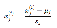
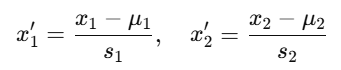
(1)均值归一化(Mean Normalization)
将特征值平移并缩放到近似于[−1,1] 的范围:
其中:
-
xj(i):第 i 个样本的第 j 个特征
-
μj:特征 j 的均值(mean)
-
sj:特征 j 的取值范围(如 max-min)
(2)Z 分数归一化(Z-score Normalization)
又称 标准化(Standardization),常用于特征分布接近高斯分布(正态分布)时:
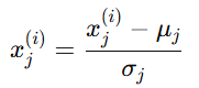
其中:
-
σj:特征 j 的标准差(standard deviation)
标准化后,数据的均值为 0,方差为 1。
3. 代码实现示例
# 均值归一化
x_scaled = (x - np.mean(x)) / (np.max(x) - np.min(x))

# Z-score 归一化
x_standardized = (x - np.mean(x)) / np.std(x)
二、梯度下降收敛(Gradient Descent Convergence)
1. 学习曲线(Learning Curve)
通过绘制 代价函数 J(w, b) 随迭代次数的变化曲线,可以观察模型是否收敛。
-
如果 J(w,b)逐渐减小并趋于平稳 → 收敛成功
-
如果 J(w,b)忽上忽下 → 学习率过大
-
如果 J(w,b) 缓慢下降 → 学习率过小
2. 自动收敛测试(Epsilon 检测)
理论上,我们可以设置一个极小的数 ϵ 来判断是否收敛:
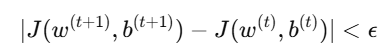
但在实践中,ϵ 很难确定。通常仍然建议:
-
通过绘图直观观察学习曲线
-
或限定最大迭代次数
3. 学习率(Learning Rate, α)的选择
(1)过小的学习率
-
每次更新步长太小
-
收敛非常慢
-
代价函数几乎不下降
(2)过大的学习率
-
每次步长过大,可能跨过最小值
-
J(w,b) 反而增大甚至震荡
-
模型永远无法收敛
(3)合适的学习率
-
J(w,b) 平滑下降并趋于稳定
-
通常通过实验确定最佳 α 值(如 0.01、0.03、0.1 等)
4. 梯度下降参数更新公式
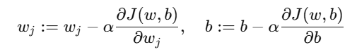
对于参数 wj 和 b,梯度下降更新规则如下:
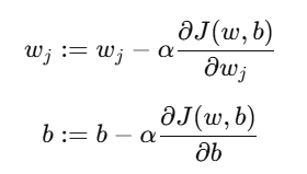
所有参数 同时更新(synchronous update)。
三、例子:房价预测中的特征缩放与梯度下降
1. 问题背景
我们想要根据两种特征预测房价:
| 特征 | 说明 | 单位 | 示例 |
|---|---|---|---|
| x1 | 房屋面积 | 平方英尺 | 2100 |
| x2 | 卧室数量 | 间 | 3 |
| y | 房价 | 美元 | 400000 |
原始数据范围相差悬殊(2100 vs 3),如果不进行特征缩放,梯度下降会非常慢。
2. 归一化处理
我们先对两个特征分别做 均值归一化:
假设:
-
房屋面积的平均值:μ1=2000,范围 s1=1000
-
卧室数量的平均值:μ2=3,范围 s2=2
则样本 (2100, 3) 转换后为:
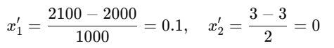
这样,所有特征值都落入 [−1,1][-1, 1][−1,1] 附近,有助于更快收敛。
3. 模型表达式
假设线性回归模型为:
![]()
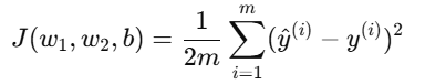
代价函数为:
4. 梯度下降过程
每一次迭代中:
设初始参数w1=w2=b=0,学习率 α=0.1,经过多次迭代后,模型逐渐逼近最优解。
5. 可视化学习曲线
import numpy as np
import matplotlib
matplotlib.use('Agg') # 使用非交互式后端
import matplotlib.pyplot as plt
# 设置中文字体
plt.rcParams['font.sans-serif'] = ['WenQuanYi Zen Hei']
plt.rcParams['axes.unicode_minus'] = False
def generate_data(n_samples=100):
"""生成线性回归的模拟数据"""
np.random.seed(42)
x = np.random.randn(n_samples, 3) * 2 # 3个特征
true_w = np.array([1.5, -2.0, 0.5]) # 真实权重
true_b = 1.0 # 真实偏置
y = x @ true_w + true_b + np.random.randn(n_samples) * 0.5 # 添加噪声
return x, y, true_w, true_b
def feature_scaling(X):
"""特征缩放(标准化)"""
return (X - np.mean(X, axis=0)) / np.std(X, axis=0)
def compute_cost(X, y, w, b):
"""计算线性回归的代价函数(均方误差)"""
m = len(y)
predictions = X @ w + b
cost = np.sum((predictions - y) ** 2) / (2 * m)
return cost
def gradient_descent(X, y, w, b, alpha, num_iters):
"""执行梯度下降算法"""
m = len(y)
J_history = []
for i in range(num_iters):
# 计算预测值
predictions = X @ w + b
# 计算梯度
dw = (1/m) * X.T @ (predictions - y)
db = (1/m) * np.sum(predictions - y)
# 更新参数
w = w - alpha * dw
b = b - alpha * db
# 记录代价函数值
cost = compute_cost(X, y, w, b)
J_history.append(cost)
# 每100次迭代打印一次进度
if i % 100 == 0:
print(f"迭代 {i}: 成本 = {cost:.6f}")
return w, b, J_history
def main():
print("=== 线性回归学习曲线示例 ===\n")
# 1. 生成数据
X, y, true_w, true_b = generate_data()
print(f"生成数据: {len(y)}个样本,{X.shape[1]}个特征")
print(f"真实参数: w = {true_w}, b = {true_b:.2f}")
# 2. 特征缩放
X_scaled = feature_scaling(X)
print("完成特征缩放(标准化)")
# 3. 初始化参数
w_init = np.zeros(X.shape[1])
b_init = 0.0
alpha = 0.01
num_iters = 100
print(f"\n梯度下降参数:")
print(f"学习率 α = {alpha}")
print(f"迭代次数 = {num_iters}")
print(f"初始参数: w = {w_init}, b = {b_init:.2f}")
# 4. 执行梯度下降
w_final, b_final, J_history = gradient_descent(
X_scaled, y, w_init, b_init, alpha, num_iters
)
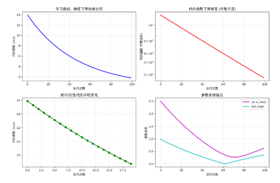
# 5. 绘制学习曲线
plt.figure(figsize=(12, 8))
# 主图:学习曲线
plt.subplot(2, 2, 1)
plt.plot(J_history, 'b-', linewidth=2)
plt.xlabel('迭代次数')
plt.ylabel('代价函数 J(w,b)')
plt.title('学习曲线 - 梯度下降收敛过程')
plt.grid(True, alpha=0.3)
# 子图1:代价函数下降速度
plt.subplot(2, 2, 2)
plt.semilogy(J_history, 'r-', linewidth=2)
plt.xlabel('迭代次数')
plt.ylabel('代价函数 (对数坐标)')
plt.title('代价函数下降速度 (对数尺度)')
plt.grid(True, alpha=0.3)
# 子图2:前20次迭代的详细变化
plt.subplot(2, 2, 3)
plt.plot(J_history[:20], 'g-', linewidth=2, marker='o')
plt.xlabel('迭代次数')
plt.ylabel('代价函数 J(w,b)')
plt.title('前20次迭代的详细变化')
plt.grid(True, alpha=0.3)
# 子图3:参数收敛情况
plt.subplot(2, 2, 4)
w_history = []
b_history = []
w_temp, b_temp = w_init.copy(), b_init
for i in range(num_iters):
predictions = X_scaled @ w_temp + b_temp
dw = (1/len(y)) * X_scaled.T @ (predictions - y)
db = (1/len(y)) * np.sum(predictions - y)
w_temp = w_temp - alpha * dw
b_temp = b_temp - alpha * db
w_history.append(np.linalg.norm(w_temp - true_w))
b_history.append(abs(b_temp - true_b))
plt.plot(w_history, 'm-', linewidth=2, label='||w-w_true||')
plt.plot(b_history, 'c-', linewidth=2, label='|b-b_true|')
plt.xlabel('迭代次数')
plt.ylabel('参数误差')
plt.title('参数收敛情况')
plt.legend()
plt.grid(True, alpha=0.3)
plt.tight_layout()
plt.savefig('learning_curve_complete.png', dpi=300, bbox_inches='tight')
print("\n学习曲线图已保存为: learning_curve_complete.png")
# 6. 结果分析
print("\n=== 训练结果分析 ===")
print(f"最终参数:")
print(f" w = {w_final}")
print(f" b = {b_final:.4f}")
print(f"最终代价函数值: {J_history[-1]:.6f}")
print(f"初始代价函数值: {J_history[0]:.6f}")
print(f"代价函数下降比例: {((J_history[0] - J_history[-1]) / J_history[0] * 100):.2f}%")
# 7. 绘制最终预测效果
plt.figure(figsize=(10, 6))
# 计算预测值
y_pred = X_scaled @ w_final + b_final
# 绘制真实值vs预测值
plt.subplot(1, 2, 1)
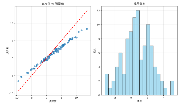
plt.scatter(y, y_pred, alpha=0.6)
plt.plot([y.min(), y.max()], [y.min(), y.max()], 'r--', linewidth=2)
plt.xlabel('真实值')
plt.ylabel('预测值')
plt.title('真实值 vs 预测值')
plt.grid(True, alpha=0.3)
# 绘制残差分布
residuals = y - y_pred
plt.subplot(1, 2, 2)
plt.hist(residuals, bins=20, alpha=0.7, color='skyblue', edgecolor='black')
plt.xlabel('残差')
plt.ylabel('频次')
plt.title('残差分布')
plt.grid(True, alpha=0.3)
plt.tight_layout()
plt.savefig('prediction_analysis.png', dpi=300, bbox_inches='tight')
print("预测效果分析图已保存为: prediction_analysis.png")
return J_history
if __name__ == "__main__":
J_history = main()
四、总结
| 概念 | 含义 | 作用 |
|---|---|---|
| 特征缩放 | 统一特征的数值范围 | 加快梯度下降收敛速度 |
| 均值归一化 | (x - mean) / (max - min) | 数据近似 [-1,1] |
| Z-score 标准化 | (x - mean) / std | 数据均值为0,方差为1 |
| 学习曲线 | 监控代价函数变化 | 判断学习率是否合适 |
| 学习率 α | 决定更新步幅 | 太大不收敛,太小太慢 |
| Epsilon 测试 | 判断收敛停止条件 | 实际中较少单独使用 |


 1401
1401

 被折叠的 条评论
为什么被折叠?
被折叠的 条评论
为什么被折叠?
 到【灌水乐园】发言


