基于FLUXNET的dryness Index(aridy Index) 和潜在蒸散发（potential evapotranspiration,PET)计算

柚柚柚子爱吃葡萄柚

已于 2024-06-14 22:54:59 修改

阅读量2k

点赞数 5

分类专栏： # 1.1 陆地生态系统碳水循环文章标签：经验分享学习

于 2022-07-30 01:06:27 首次发布

本文链接：https://blog.csdn.net/Wangxr_cau/article/details/126065639

版权

1.1 陆地生态系统碳水循环专栏收录该内容

2 篇文章 0 订阅

订阅专栏

文章内容仅用于自己知识学习和分享，如有侵权，还请联系并删除：）

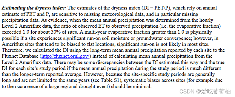
（一）Dryness Index(aridy Index) 计算

在这里插入图片描述

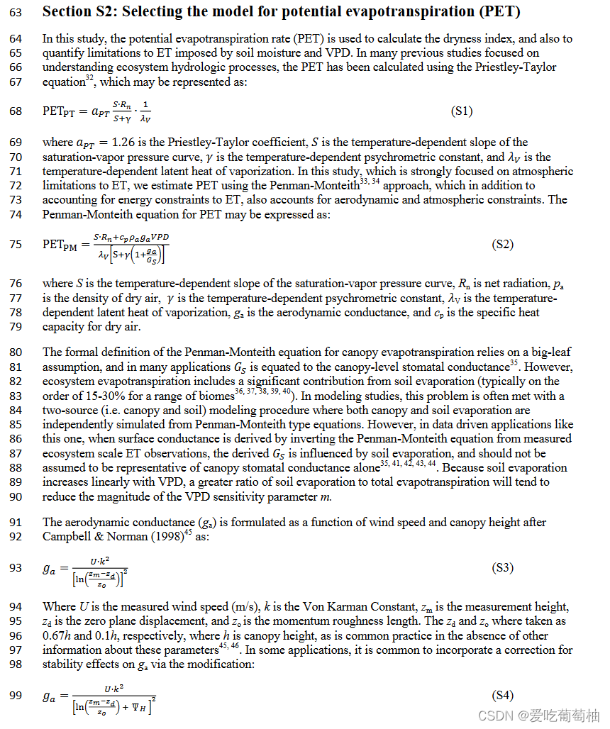
（二）PET计算

1. 英文描述

见参考文献[1-3] , 作者计算PET使用了两种方法，分别是Priestley-Taylor和Penman-Monteith
[1] link ；[2] link；[3] link
在这里插入图片描述

2. 中文描述

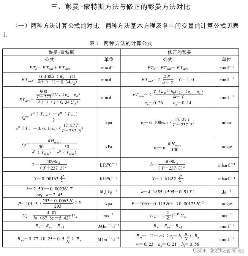
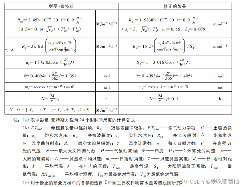
彭曼公式参数定义见参考文献[4] link

3. R计算包

见参考文献[5]

官方文档： link
对应的论文：link
安装指南：link

（1）原理简介

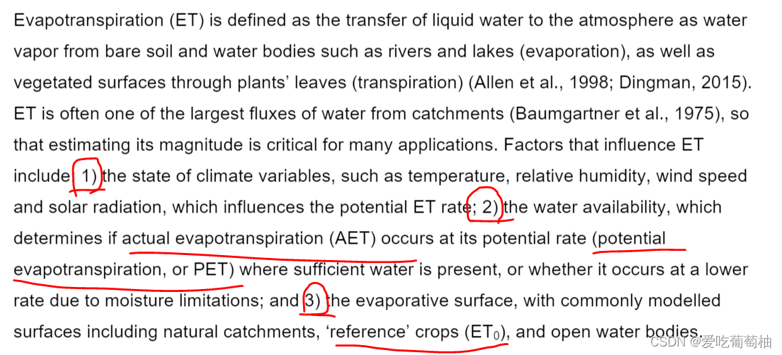
该R package包含17个常用的计算actual ET（AET）, potential ET (PET) and reference ET (ET0）模型（ps:关于potential和reference的区别，B站有视频讲解）
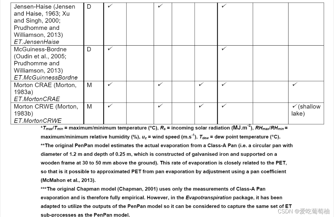
17个模型分别是：

– The equations for 15 ET models included in the package (all models except for Jensen-Haise and McGuinness-Bordne) are sourced from McMahon et al. (2013), which have allbeen verified with examples presented in their original paper.

– For the other two structurally simple models, Jensen-Haise andMcGuinness-Bordne, which are sourced from Prudhomme and Williamson (2013), there areno published examples of implementation available for verification.
在这里插入图片描述

R package主要函数

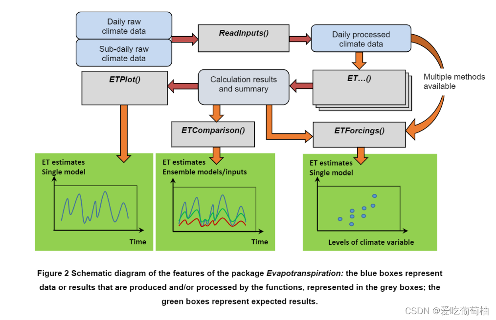
代码的调用主要包含以下五个步骤：

第一步：数据预处理 The data pre-processing function ReadInputs() is developed for loading and processing sub-daily and daily raw climate data.

ReadInputs()该函数主要包括三个功能：（1）检查data availability; (2) 识别missing entries; (3) 检查异常值

（1）检查data availability
在这里插入图片描述

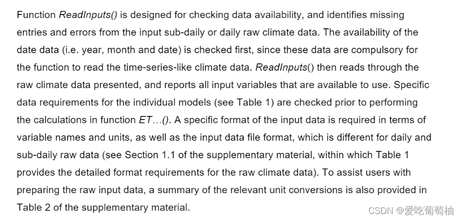
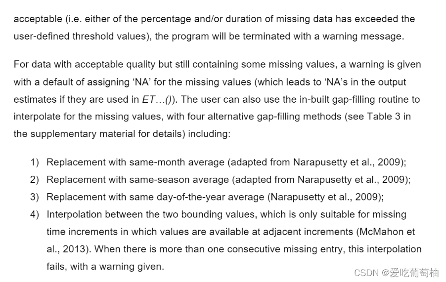
（2）识别missing entries
在这里插入图片描述

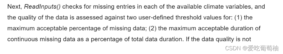
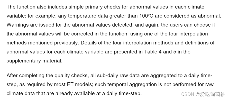
（3）检查异常值

在这里插入图片描述
第二步:指定ET模型计算方法， generic function ET…(), where each of the 17 different methods canbe called by substituting the ‘…’ by the function name (e.g. ‘ET.Penman ()’ to call the Penman model). The function performs calculations for the relevant ET model and generatesa calculation summary.

（1）如果输入数据不满足指定ET模型，代码会自动选择可替代的模型，如果没有可替代的模型，代码会给出warning

在这里插入图片描述

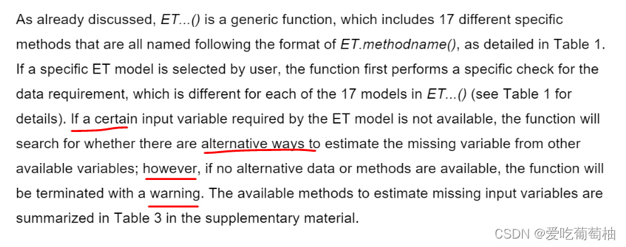
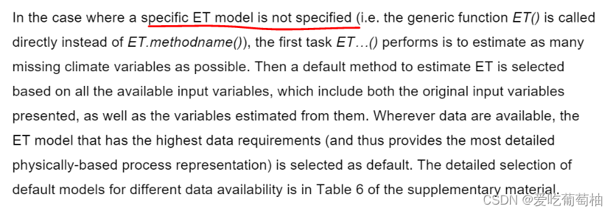
（2）如果没有指定ET模型，会使用默认模型计算

在这里插入图片描述

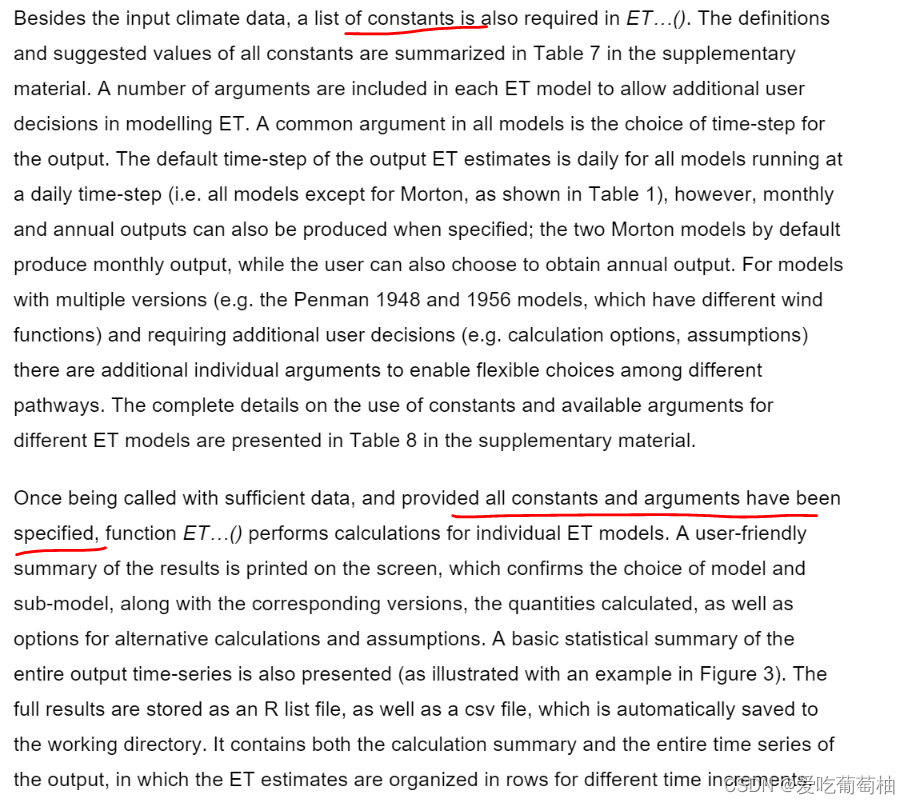
（3）模型除了需要输入气象变量，还需要指定固定参数，固定参数取值见附录Table7，代码已经进行了默认设置；一旦模型成功运行，会在working directory下自动生成R文件或者csv文件

在这里插入图片描述
第三步：画图，可以画出不同时间尺度的计算得到的ET，: Having calculated the ET quantity, the function ETPlot() can then be called to plot the original estimates, as well as aggregations and averages at different time scales.

A number of plotting tools are available to analyse the outputs. Function ETPlot() uses theestimated daily ET from individual ET models to generate aggregation plots and averageplots at daily, monthly and annual time steps

第四步:结果比较， FunctionETComparison() facilitates comparison of results and visualization of uncertainties fromusing different models and/or different input data.

Function ETComparison() producescomparison plots of different sets of ET estimates, to compare the outputs from :

(1) different ET models; （不同ET模型）
(2) different versions of the same ET model (e.g. the 1948 and 1956 versions of the Penman model); （同一ET模型不同版本）
(3) the same ET model with different calculation options, such as alternative approaches for data infilling and/or; （同一ET模型，但是不同计算选项）
(4) different sets of input climate data. Foreach quantity, three types of plots, including: time series plots, non-exceedance probabilityplots and box plots, can be produced. (不同出图方式）
(5) Plots of uncertainty ranges can also be produced for daily estimates, monthly and annual aggregates and monthly and annual averages. (不确定性范围）

第五步:比较输入气象变量和计算得到的ET之间的关系， ETForcing() enables the association between estimated ET and different climate variables to be plotted.

The function ETForcing() is an additional plotting tool for visualizing the association between estimated ET and different climate variables within existing data.

（2）安装

作者还提供了一个站点使用案例，可参考其论文

install.packages('Evapotranspiration')

（3）尝试使用FLUXNET 数据计算PET

以US-MMS为例，下图为参考文献[1] link ；[2] link；计算得到的结果，[1] 使用彭曼（PM）公式，[2] 使用Priestley-Taylor（PT）公式，这里使用Priestley-Taylor （PT）公式计算
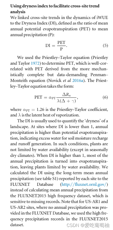
图1为基于PM公式计算得到的dryness Index=1.43
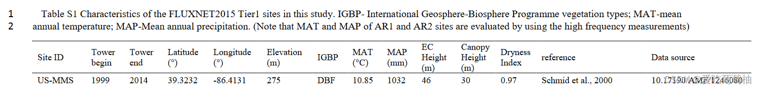
图2为基于PT公式计算得到的dryness Index=0.97
PT计算公式如下

中文定义：下面这个公式是不是少了一个γ？[8] link
在这里插入图片描述

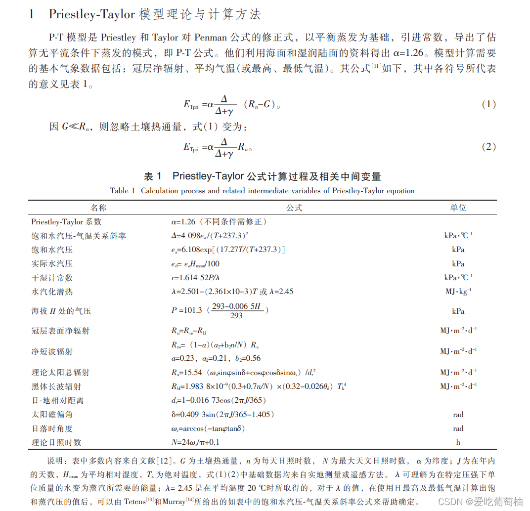
中文定义： [9] link

在这里插入图片描述

~~~~~~~~~~~~~~~~~~~~~~~~~~~~~~~~~~~~~~~~~~~~~~~~~~~~~~~

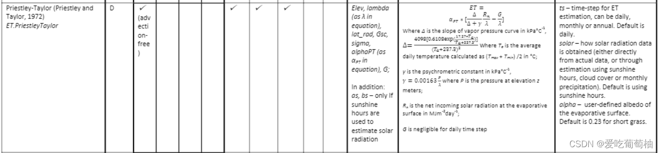
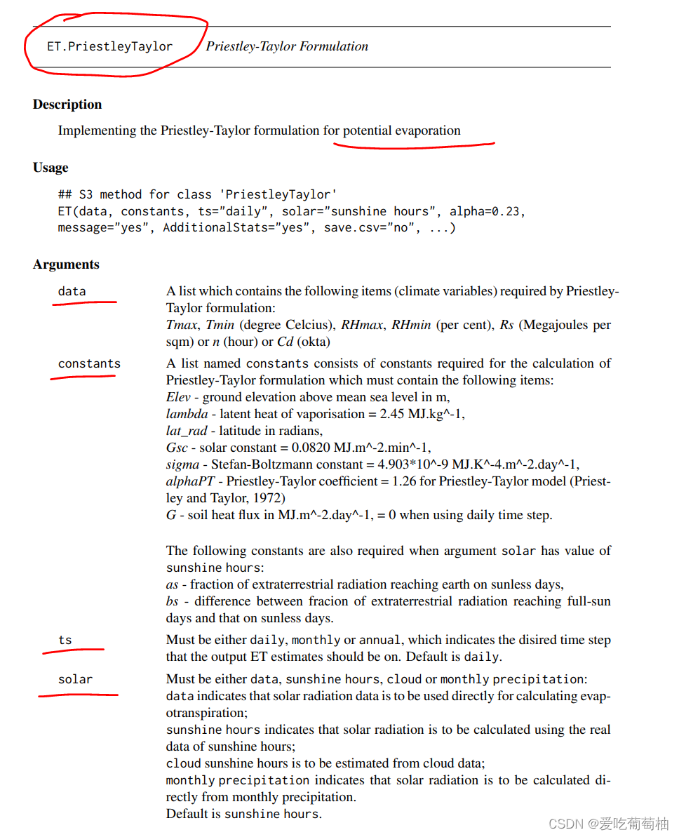
（3-1） R 包中计算公式和参数设置

（1）R中的计算公式
在这里插入图片描述
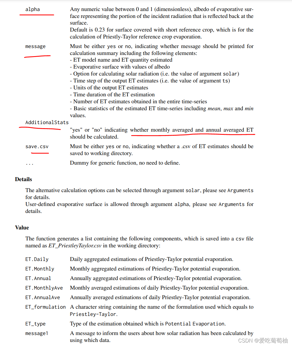
（2）函数输入输出变量

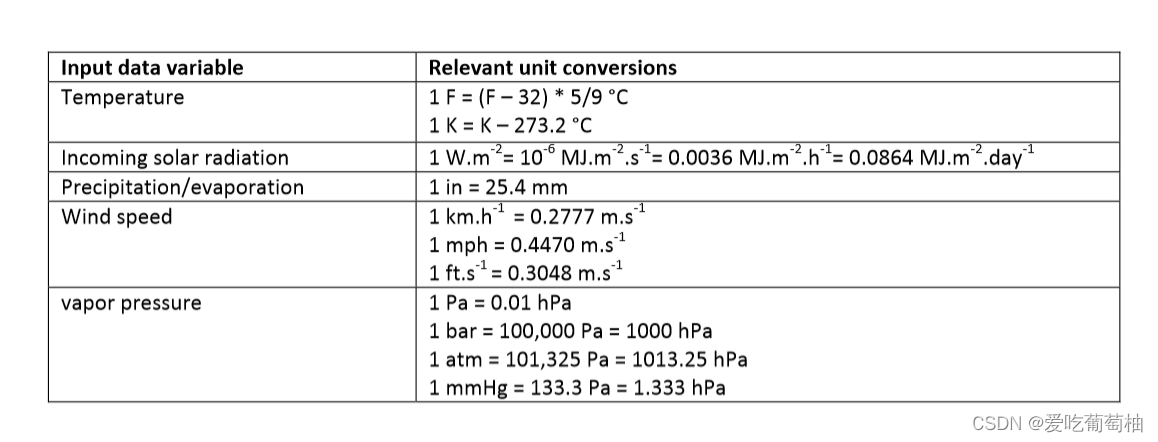
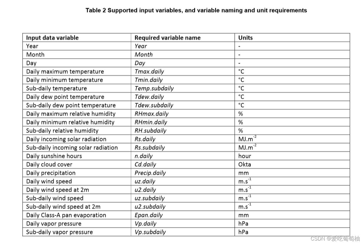
（3）单位转换及其变量名定义
在这里插入图片描述

// 注意点：
#目标： 使用Priestley-Taylor计算US-MMS站点的年潜在PET

[1] 输入气象变量：日最低/高温度，日最低/高RH,太阳辐射
由上述函数可知，模型需要输入日最高/最低 气温和相对湿度，以及冠层净辐射，最高最低值主要用来计算日均温和日相对指数，因此如果已经由日均温和日相对湿度，那就直接把这两个变量传给代码就行，因为模型求均温时候是求了最低和最高温的均值
- 参数单位：
- （1）辐射要把w/m2,转换成 MJ/m2/d,  1MJ=1000000J，w/m2= J/m2/s, MJ/m2/d=24*60*60 *w/m2 /1000000
- 单位转换参考链接： 
http://www.endmemo.com/sconvert/w_m2j_sm2.php
https://stackoverflow.com/questions/40826466/solar-energy-conversion-w-m2-to-mj-m2
	 Example： Your panels do 294 Watt per m², i.e. 294 Joule per sec per m². So that's 24*60*60 * 294 = 25401600 Joule per m² per day, or 25.4016 MJ per m² per day.A watt is the unit of power and Joules are the units of energy, they are related by time. 1 watt is 1 Joule per second 1W = 1 J/s. So the extension of that equation is that 1J = 1w x 1second. 1J = 1Ws
- （2）VPD转换成相对湿度RH(kpa->%)

[2] 输入常数
Priestley-Taylor formulation which must contain the following items:
(1) Elev - ground elevation above mean sea level in m,(US-MMS elevation = 275m)
(2) lambda - latent heat of vaporisation = 2.45 MJ.kg^-1,
(3) lat_rad - latitude in radians,(US-MMS latitude = 39.32*180/pi)
(4) Gsc - solar constant = 0.0820 MJ.m^-2.min^-1,
(5) sigma - Stefan-Boltzmann constant = 4.903*10^-9 MJ.K^-4.m^-2.day^-1,
(6) alphaPT - Priestley-Taylor coefficient = 1.26 for Priestley-Taylor model (Priestley and Taylor, 1972)
(7) G - soil heat flux in MJ.m^-2.day^-1, = 0 when using daily time step.



# -------------------------------------------------
# FUNCTION: calculate potential ET an dryness Index (=annual PET/ annual Precipitation)
# Date: 2022/08/01

# 1. climate data
# TA_F_MDS:degree
# VPD: kpa
# RH: % 
# NETRAD: w/m2
# Rs.daily: MJ/m2/d

# 2. constants
# Priestley-Taylor formulation which must contain the following items:
# (1) Elev - ground elevation above mean sea level in m,(US-MMS elevation = 275m)
# (2) lambda - latent heat of vaporisation = 2.45 MJ.kg^-1,
# (3) lat_rad - latitude in radians,(US-MMS latitude = 39.32*180/pi)
# (4) Gsc - solar constant = 0.0820 MJ.m^-2.min^-1,
# (5) sigma - Stefan-Boltzmann constant = 4.903*10^-9 MJ.K^-4.m^-2.day^-1,
# (6) alphaPT - Priestley-Taylor coefficient = 1.26 for Priestley-Taylor model (Priestley and Taylor, 1972)
# (7) G - soil heat flux in MJ.m^-2.day^-1, = 0 when using daily time step.
# -----------------------------------




# install.packages('Evapotranspiration') #PET calculation
# install.packages('naniar') # -9999<-NaN
# install.packages('plantecophys') #VPD<-RH

library(Evapotranspiration)
library(naniar)  
library(plantecophys) 

setwd(".../Process during vacation")

# step1: Read data 
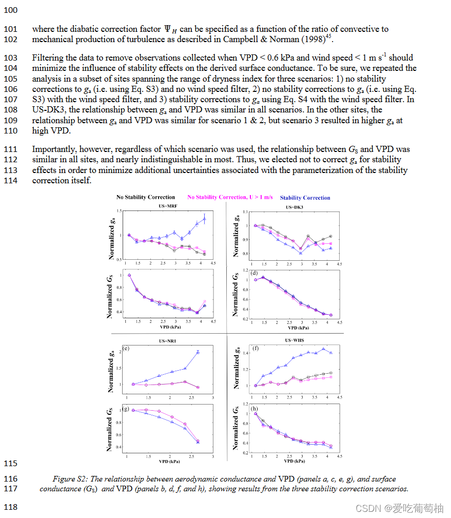
df <- read.csv(file = '.../FLX_US-MMS_FLUXNET2015_FULLSET_DD_1999-2014_1-4.csv')


# step2:replace -9999 as NaN
df <- df%>%replace_with_na_all(condition = ~.x == -9999)


# step3:Define the input dataset
Year<-floor(df$TIMESTAMP/10000)
Month<-floor((df$TIMESTAMP-Year*10000)/100)
Day<-floor(df$TIMESTAMP-Year*10000-Month*100)
Tmax.daily<-df$TA_F_MDS 
Tmin.daily<-df$TA_F_MDS 
RH<-VPDtoRH(df$VPD_F, df$TA_F_MDS, Pa = 101)
RHmax.daily= RH  
RHmin.daily= RH 
#Rs.daily = (df$NETRAD)*24*60*60/1000000
Rs.daily = (df$SW_IN_F_MDS)*24*60*60/1000000

climatedata = data.frame(
  Year = Year,
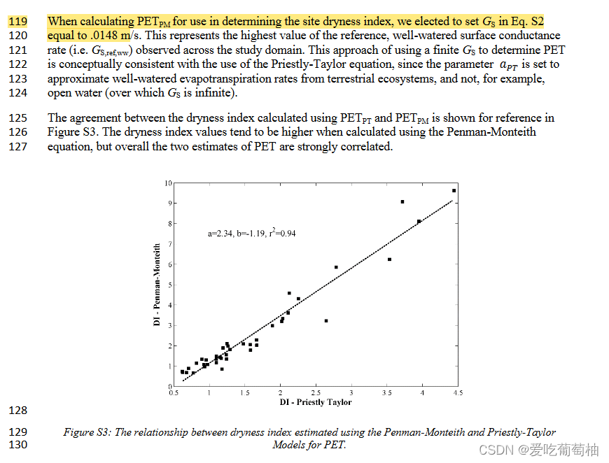
  Month= Month,
  Day  = Day,
  Tmax =Tmax.daily,
  Tmin =Tmin.daily,
  RHmax=RHmax.daily,
  RHmin=RHmin.daily,
  Rs= Rs.daily
)

constants = data.frame(
  Elev = 275,
  lambda = 2.45,
  lat_rad = 39.32*180/pi,
  Gsc = 0.082,
  sigma = 4.903/1000000000,
  alphaPT = 1.26,
  G =0
)

#step4: checkinput data


data <- ReadInputs(
                   varnames = c("Year","Month","Day","Tmax","Tmin","RHmax","RHmin","Rs"),
                   climatedata,
                   constants,
                   stopmissing=c(10,10,3),
                   timestep = "daily",
                   interp_missing_days = FALSE,
                   interp_missing_entries = FALSE,
                   interp_abnormal = FALSE,
                   missing_method = NULL,
                   abnormal_method = NULL)


#step5: calculate potential ET
Results<-ET(data, constants, ts="daily", solar='data', alpha=0.23,
   message="yes", AdditionalStats="yes", save.csv="yes")

file.rename(from='ET_PriestleyTaylor.csv', to='US_MMS_ET_PriestleyTaylor.csv')

（三）Reference

[1] Supplementary Information and Discussion for “The increasing importance of atmospheric demand for ecosystem water and carbon fluxes”: link
[2] Response of ecosystem intrinsic water use efficiency and gross primary productivity to rising vapor pressure deficit: link
Supplementary “Response of ecosystem intrinsic water use efficiency and gross primary productivity to rising vapor pressure deficit”: link
[3] Global divergent responses of primary productivity to water, energy, and CO2: link
[4] MATLAB利用不同方法实现潜在蒸散发计算: link
[5] R package:

官方文档： link
对应的论文：link
安装指南：link

[6] FLUXNET站点经纬度和年降水： link
[7] 使用EToCalculator 计算潜在蒸散发详细教程: link
[8] Priestly-Taylor 模型参数修正及在蒸散发估算中的应用：link
[9] 参照腾发量的新定义及计算方法对比: link
[10] Package ‘plantecophys’ link,可以进行VPD和RH的转换

柚柚柚子爱吃葡萄柚

关注

5
点赞
踩
19

收藏

觉得还不错? 一键收藏
3
评论
基于FLUXNET的dryness Index(aridy Index) 和潜在蒸散发（potential evapotranspiration,PET)计算

生态，FLUXNET, 潜在蒸散发,dryness Index
复制链接

扫一扫