


Stanford公开课Exercise 3原题地址:http://openclassroom.stanford.edu/MainFolder/DocumentPage.php?course=MachineLearning&doc=exercises/ex3/ex3.html,下面是我完成的笔记。
第一部分,gradient descent方法
(一)原理回顾
简单重复一下gradient descent实现的过程,具体的看前面的文章(【机器学习笔记2】Linear Regression总结):
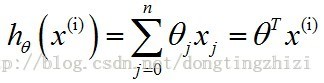
1. h(θ)函数
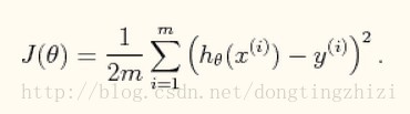
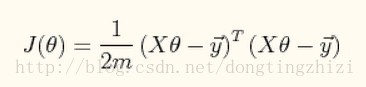
2. J(θ)函数
向量化后简化为:
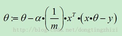
3. θ迭代过程
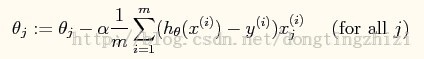
向量化后简化为:
4. Feature Scaling
 (公式6)
(公式6)
(二)实现代码
- %=================================================================
- % Exercise 3: Multivariate Linear Regression (gradient descent)
- % author : liubing (liubing80386@163.com)
- %
- %LB_c: 加载数据 ===============
- x = load("ex3x.dat");
- y = load("ex3y.dat");
- %LB_c: 矩阵x第一列加上全1
- x = [ones(size(x)(1),1), x];
- %==============================
- %LB_c: scaling(缩放到相同范围),参考上面的(公式6)
- sigma = std(x); %x按列求标准差
- mu = mean(x); %x按列求均值
- %第2、3列scaling(第1列全为1,不用做)
- x(:,2) = (x(:,2) - mu(2)) ./ sigma(2);
- x(:,3) = (x(:,3) - mu(3)) ./ sigma(3);
- %==================================================
- %LB_c: 常量数据准备=============================================================
- %theta更新的迭代次数
- iter_total = 50;
- %m为样本数,n为特征数(包含第一列的常数项,实际特征数为n-1)
- [m,n] = size(x);
- %学习率的不同取值,共7个,实验结果表明前6个收敛,最后一个发散
- alpha = [0.01, 0.03, 0.1, 0.3, 1, 1.3, 1.4];
- %对应不同学习率结果绘制的属性
- plot_arg = ['c', 'r', 'g', 'b', 'm', 'k', 'r', 'b'];
- alpha_total = length(alpha); %不同学习率种数
- theta_arr = zeros(alpha_total, n); %存储所有alpha值对应的theta结果
- %===============================================================================
- %LB_c ==========================================================================
- %尝试不同的alpha值,绘制J值迭代趋势,theta结果保存到theta_arr中
- figure;
- title("J(theta) converge");
- xlabel('iteration (times)');
- ylabel('J(theta)');
- for alpha_index = [1:alpha_total]
- theta = zeros(n,1); %theta初始化为全0,其他值也可以
- J = zeros(iter_total,1); %存储每一步迭代的J(theta)值
- %迭代过程
- for iter_index = [1:iter_total]
- J(iter_index) = (x*theta-y)' * (x*theta-y) / (2*m); %求当前的J(theta),参考上面的(公式3)
- err = x * theta - y;
- grad = ( x' * err ) / m; %求gradient
- theta = theta - alpha(alpha_index) * grad; %梯度下降法更新theta,参考上面的(公式5)
- end
- %保存当前alpha的theta结果
- theta_arr(alpha_index,:) = theta';
- %绘制当前alpha的J值迭代趋势
- if ( alpha_index == 7 )
- legend('0.01', '0.03', '0.1', '0.3', '1', '1.3');
- figure;
- title("J(theta) diverge");
- xlabel('iteration (times)');
- ylabel('J(theta)');
- end
- hold on;
- plot([0:49], J, plot_arg(alpha_index), 'LineWidth', 2);
- %a = input("continue : ");
- end
- legend('1.4');
- %===============================================================================
- %LB_c:结果输出 ======================================================================
- alpha = theta_arr(5);
- printf("theta for alpha=1 : \n");
- theta_arr(5,:)
- test_x = [1, 1650, 3]; %测试数据
- test_x(2) = (test_x(2) - mu(2)) / sigma(2); %scaling
- test_x(3) = (test_x(3) - mu(3)) / sigma(3); %scaling
- predict_price = test_x * theta_arr(5,:)'; %计算预测值
- printf("predicted price for test data(1650-square-foot house with 3 bedrooms) : \n");
- predict_price
- %=====================================================================================
(三)执行结果
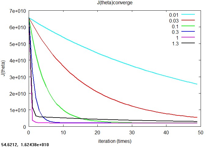
1. J(θ)收敛的情况,改图对比了当学习率α分别为0.01、0.03、0.1、0.3、1和1.3时J(θ)的收敛趋势,根据对比来选择合适的学习率。本例中,因为α为1时收敛最快而且效果相当,所以选择了α为1。
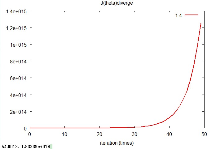
2. J(θ)发散的情况,当α为1.4时,J(θ)发散的非常厉害,而且实验中发现当α为1.5,1.6甚至更大时发散更加快,J(θ)甚至相差多个数量级,无法在一个图中绘制出来。由此可以看出,α的选取在gradient descent中是非常重要的。
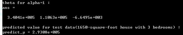
3. 下面是一些输出结果:当α=1时最终求得的回归系数theta,并用该theta值预测题目中给出的测试例子(1650平米,3个卧室),得到的预测房价。得到的结果与题目中给出的solution基本一致。
第二部分,normal equation方法
原题还要求用normal equation实现,并与gradient descent方法进行对比。normal equation的实现很简单,就是前面的文章(【机器学习笔记2】Linear Regression总结)中提到的公式:
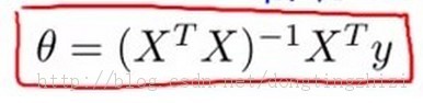
实现代码如下:
- %=================================================================
- % Exercise 3: Multivariate Linear Regression (normal equation)
- % author : liubing (liubing80386@163.com)
- %
- %LB_c: 加载数据 ===============
- x = load("ex3x.dat");
- y = load("ex3y.dat");
- %LB_c: 矩阵x第一列加上全1
- x = [ones(size(x)(1),1), x];
- %==============================
- theta = inv(x'*x)*x'*y; %normal equation,参考上面的(公式7)
- test_x = [1, 1650, 3]; %测试数据
- price = test_x * theta; %计算预测值
- printf("theta from normal equation : \n");
- theta
- printf("predicted price for test data(1650-square-foot house with 3 bedrooms) : \n");
- price
执行结果
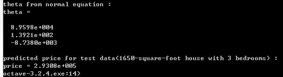
可以看出,normal equation方法得到的预测值与gradient descent方法得到的是一样(2.9308e+005)。


 626
626

 被折叠的 条评论
为什么被折叠?
被折叠的 条评论
为什么被折叠?
 到【灌水乐园】发言


