


Tensorflow2程序设计案例
1.单层神经网络-Fashion-MNIST
1.1目标与步骤
本题完成解析图片识别时尚衣服单品的功能,以此达到或者掌握Tensorflow2的单层神经网络的知识点。
实施步骤如下:
1:准备数据如数据源所示,
据由一些图片构成,里面的内容是时尚单品;
2:利用Tensorflow2单层神经网络推断出图片分类代表0-9中的哪个类别,首先收集导入Tensorflow2的支持,加载数据集,浏览数据,预处理数据,构建模型,编译模型,训练模型,评估模型,预测模型,详细代码见5.1.3所示;
3:代码编写完成之后,可以直接在jupyter notebook上运行;或者是将代码保存为py文件,使用python3命令在本机运行,提交过程如5.1.4所示;
4;最终计算之后得到的结果文件如5.1.5所示;
3.1.2数据源
FashionMNIST 是一个替代 MNIST 手写数字集 的图像数据集。 它是由 Zalando(一家德国的时尚科技公司)旗下的研究部门提供。其涵盖了来自 10 种类别的共 7 万个不同商品的正面图片。
FashionMNIST 的大小、格式和训练集/测试集划分与原始的 MNIST 完全一致。60000/10000 的训练测试数据划分,28x28 的灰度图片。你可以直接用它来测试你的机器学习和深度学习算法性能,且不需要改动任何的代码。
标注编号描述
0:T-shirt/top(T恤)
1:Trouser(裤子)
2:Pullover(套衫)
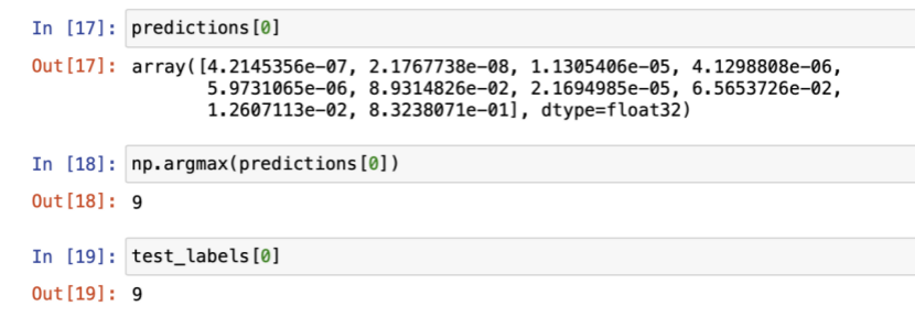
3:Dress(裙子)
4:Coat(外套)
5:Sandal(凉鞋)
6:Shirt(汗衫)
7:Sneaker(运动鞋)
8:Bag(包)
9:Ankle boot(踝靴)
3.1.3编码实现
1.导入tf.keras
import tensorflow as tf
from tensorflow import keras
import numpy as np
import matplotlib.pyplot as plt
print(tf.__version__)
2.加载数据集
fashion_mnist = keras.datasets.fashion_mnist
(train_images, train_labels), (test_images, test_labels) = fashion_mnist.load_data()
#每个图像都会被映射到一个标签
class_names = ['T-shirt/top', 'Trouser', 'Pullover', 'Dress', 'Coat',
               'Sandal', 'Shirt', 'Sneaker', 'Bag', 'Ankle boot']
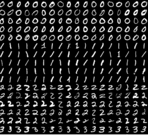
3.浏览数据
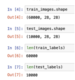
plt.figure(figsize=(10,10))
for i in range(25):
    plt.subplot(5,5,i+1)
    plt.xticks([])
    plt.yticks([])
    plt.grid(False)
    plt.imshow(train_images[i], cmap=plt.cm.binary)
    plt.xlabel(class_names[train_labels[i]])
plt.show()
4.预处理数据
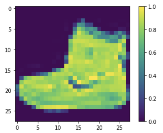
plt.figure()
plt.imshow(train_images[0])
plt.colorbar()
plt.grid(False)
plt.show()
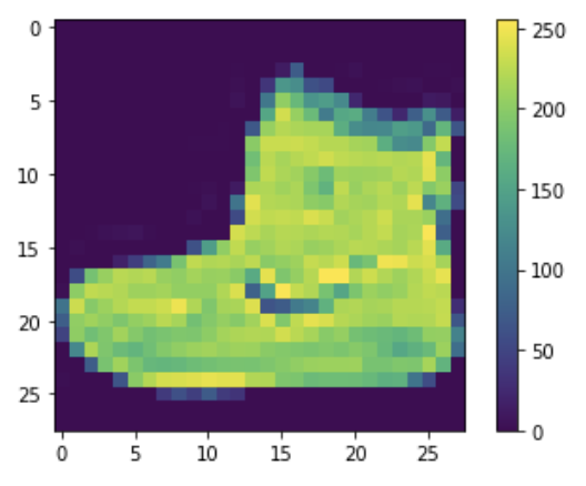
train_images = train_images / 255.0
test_images = test_images / 255.0
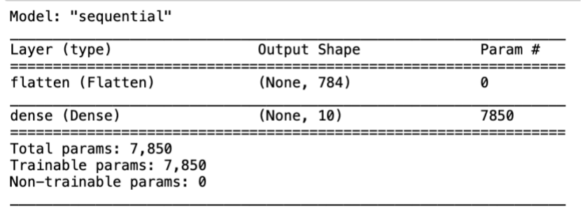
5.构建模型
model = keras.Sequential([
    keras.layers.Flatten(input_shape=(28, 28)),
    #keras.layers.Dense(128, activation='relu'),
    keras.layers.Dense(10)
])
model.summary()
6.编译模型
在准备对模型进行训练之前,还需要再对其进行一些设置。以下内容是在模型的编译步骤中添加的:
1.损失函数 - 用于测量模型在训练期间的准确率。您会希望最小化此函数,以便将模型“引导”到正确的方向上。
2.优化器 - 决定模型如何根据其看到的数据和自身的损失函数进行更新。
3.指标 - 用于监控训练和测试步骤。以下示例使用了准确率,即被正确分类的图像的比率。
model.compile(optimizer='adam',
              loss=tf.keras.losses.SparseCategoricalCrossentropy(from_logits=True),
              metrics=['accuracy'])
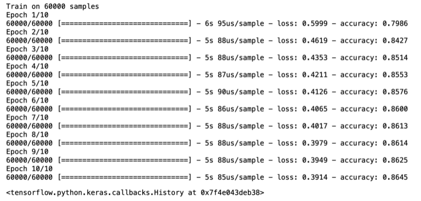
7.训练模型
训练神经网络模型需要执行以下步骤:
将训练数据馈送给模型。在本例中,训练数据位于 train_images 和 train_labels 数组中。
模型学习将图像和标签关联起来。
要求模型对测试集(在本例中为 test_images 数组)进行预测。
验证预测是否与 test_labels 数组中的标签相匹配。
model.fit(train_images, train_labels, epochs=10)
8.评估准确率
test_loss, test_acc = model.evaluate(test_images,  test_labels, verbose=2)
print('\nTest accuracy:', test_acc)
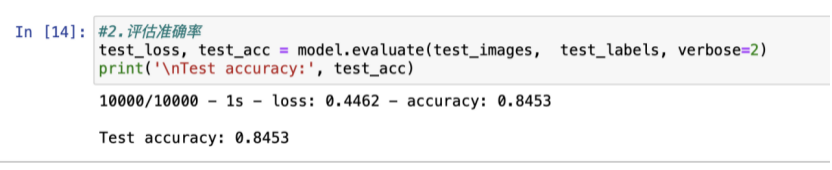
结果表明,模型在测试数据集上的准确率略低于训练数据集。训练准确率和测试准确率之间的差距代表过拟合。过拟合是指机器学习模型在新的、以前未曾见过的输入上的表现不如在训练数据上的表现。过拟合的模型会“记住”训练数据集中的噪声和细节,从而对模型在新数据上的表现产生负面影响。
9.预测模型
probability_model = tf.keras.Sequential([model, tf.keras.layers.Softmax()])
predictions = probability_model.predict(test_images)
def plot_image(i, predictions_array, true_label, img):
predictions_array, true_label, img = predictions_array, true_label[i], img[i]
plt.grid(False)
plt.xticks([])
plt.yticks([])
plt.imshow(img, cmap=plt.cm.binary)
predicted_label = np.argmax(predictions_array)
if predicted_label == true_label:
color = 'blue'
else:
color = 'red'
plt.xlabel("{} {:2.0f}% ({})".format(class_names[predicted_label],
100*np.max(predictions_array),
class_names[true_label]),
color=color)
def plot_value_array(i, predictions_array, true_label):
predictions_array, true_label = predictions_array, true_label[i]
plt.grid(False)
plt.xticks(range(10))
plt.yticks([])
thisplot = plt.bar(range(10), predictions_array, color="#777777")
plt.ylim([0, 1])
predicted_label = np.argmax(predictions_array)
thisplot[predicted_label].set_color('red')
thisplot[true_label].set_color('blue')
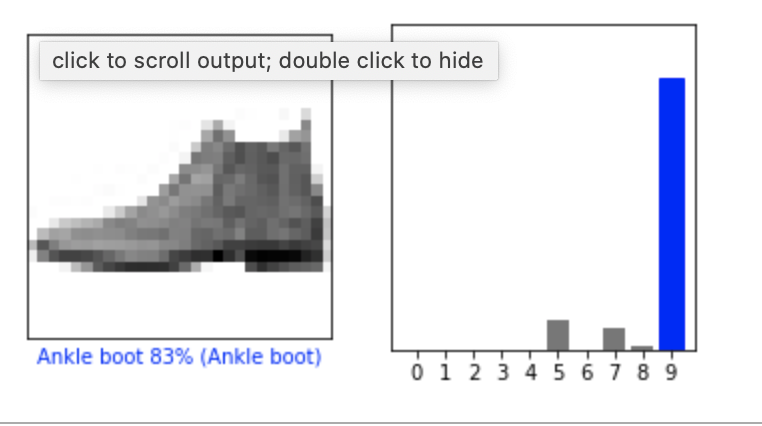
#.验证预测结果 0 12号商品
i = 0
plt.figure(figsize=(6,3))
plt.subplot(1,2,1)
plot_image(i, predictions[i], test_labels, test_images)
plt.subplot(1,2,2)
plot_value_array(i, predictions[i], test_labels)
plt.show()
3.1.4结果展示

2.多层前向神经网络-mnist
2.1目标与步骤
本题完成解析手写数字识别的功能,以此达到或者掌握Tensorflow2的多层前向神经网络的知识点。
实施步骤如下:
1:准备数据如数据源所示,数据由一些图片构成,里面的内容是手写数字;
2:利用Tensorflow2单层神经网络推断出图片分类代表0-9中的哪个类别,首先收集导入Tensorflow2的支持,加载数据集,浏览数据,预处理数据,构建模型,编译模型,训练模型,评估模型,预测模型,详细代码见3.1.3所示;
3:代码编写完成之后,可以直接在jupyter notebook上运行;或者是将代码保存为py文件,使用python3命令在本机运行;
4;最终计算之后得到的结果文件如3.1.4所示;
3.2.2数据源
手写数字矩阵的图片
3.2.3编码实现
1.导入tf.keras
import os
import tensorflow as tf
from tensorflow import keras
from tensorflow.keras import datasets, layers, optimizers
import numpy as np
2.加载数据集
data_path = os.path.abspath(os.path.dirname('.')) + '/data/mnist.npz'
(x_train, y_train), (x_test, y_test)= tf.keras.datasets.mnist.load_data(data_path)
3.指定训练参数
num_classes = 10 # 所有类别(数字 0-9)
num_features = 784 # 数据特征数目 (图像形状: 28*28)
learning_rate = 0.001
training_steps = 5000
batch_size = 256
display_step = 100
n_hidden_1 = 128 # 第一层隐含层神经元的数目
n_hidden_2 = 256 # 第二层隐含层神经元的数目
4.预处理数据
转化为float32
x_train, x_test = np.array(x_train, np.float32), np.array(x_test, np.float32)
将每张图像展平为具有784个特征的一维向量(28 * 28)
x_train, x_test = x_train.reshape([-1, num_features]), x_test.reshape([-1, num_features])
将图像值从[0,255]归一化到[0,1]
x_train, x_test = x_train / 255., x_test / 255.
使用tf.data API对数据进行随机排序和批处理
train_data = tf.data.Dataset.from_tensor_slices((x_train, y_train))
train_data = train_data.repeat().shuffle(5000).batch(batch_size).prefetch(1)
5.构建模型
存储层的权重和偏置
随机值生成器初始化权重
random_normal = tf.initializers.RandomNormal()
weights = {
    'h1': tf.Variable(random_normal([num_features, n_hidden_1])),
    'h2': tf.Variable(random_normal([n_hidden_1, n_hidden_2])),
    'out': tf.Variable(random_normal([n_hidden_2, num_classes]))
}
biases = {
    'b1': tf.Variable(tf.zeros([n_hidden_1])),
    'b2': tf.Variable(tf.zeros([n_hidden_2])),
    'out': tf.Variable(tf.zeros([num_classes]))
}
创建模型
def neural_net(x):
    # Hidden fully connected layer with 128 neurons.
    # 具有128个神经元的隐含完全连接层
    layer_1 = tf.add(tf.matmul(x, weights['h1']), biases['b1'])
    # Apply sigmoid to layer_1 output for non-linearity.
    # 将sigmoid用于layer_1输出以获得非线性
    layer_1 = tf.nn.sigmoid(layer_1)

    # 具有128个神经元的隐含完全连接层
    layer_2 = tf.add(tf.matmul(layer_1, weights['h2']), biases['b2'])
    # 将sigmoid用于layer_2输出以获得非线性
    layer_2 = tf.nn.sigmoid(layer_2)

    # 输出完全连接层,每一个神经元代表一个类别
    out_layer = tf.matmul(layer_2, weights['out'])
    biases['out']
    # 应用softmax将输出标准化为概率分布
    return tf.nn.softmax(out_layer)
6.定义损失函数
def cross_entropy(y_pred, y_true):
    # 将标签编码为独热向量
    y_true = tf.one_hot(y_true, depth=num_classes)
    # 将预测值限制在一个范围之内以避免log(0)错误
    y_pred = tf.clip_by_value(y_pred, 1e-9, 1.)
    # 计算交叉熵
    return tf.reduce_mean(-tf.reduce_sum(y_true * tf.math.log(y_pred)))
7.定义准确率评估函数
def accuracy(y_pred, y_true):
     # 预测类是预测向量中最高分的索引(即argmax)
    correct_prediction = tf.equal(tf.argmax(y_pred, 1), tf.cast(y_true, tf.int64))
return tf.reduce_mean(tf.cast(correct_prediction, tf.float32), axis=-1)
8.开启训练
随机梯度下降优化器
optimizer = tf.optimizers.SGD(learning_rate)
优化过程
def run_optimization(x, y):
    # 将计算封装在GradientTape中以实现自动微分
    with tf.GradientTape() as g:
        pred = neural_net(x)
        loss = cross_entropy(pred, y)

    # 要更新的变量,即可训练的变量
    trainable_variables = weights.values()
    biases.values()

    # 计算梯度
    gradients = g.gradient(loss, trainable_variables)

    # 按gradients更新 W 和 b
    optimizer.apply_gradients(zip(gradients, trainable_variables))
针对给定步骤数进行训练
for step, (batch_x, batch_y) in enumerate(train_data.take(training_steps), 1):
    # 运行优化以更新W和b值
    run_optimization(batch_x, batch_y)

    if step % display_step == 0:
        pred = neural_net(batch_x)
        loss = cross_entropy(pred, batch_y)
        acc = accuracy(pred, batch_y)
        print("step: %i, loss: %f, accuracy: %f" % (step, loss, acc))
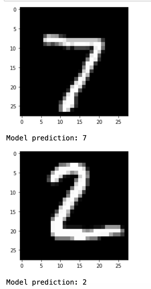
9.验证模型
可视化预测
import matplotlib.pyplot as plt
从验证集中预测5张图像
n_images = 5
test_images = x_test[:n_images]
predictions = neural_net(test_images)
显示图片和模型预测结果
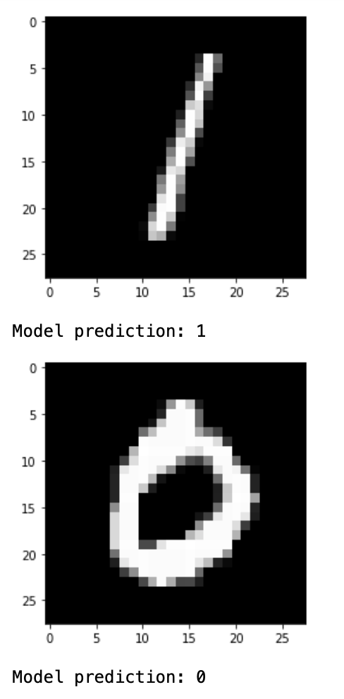
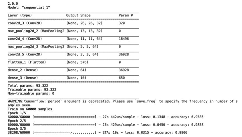
for i in range(n_images):
    plt.imshow(np.reshape(test_images[i], [28, 28]), cmap='gray')
    plt.show()
    print("Model prediction: %i" % np.argmax(predictions.numpy()[i]))
3.2.4结果展示
3.卷积神经网络-mnist
3.1目标与步骤
本题完成解析手写数字识别的功能,以此达到或者掌握Tensorflow2的卷积神经网络的知识点。
实施步骤如下:
1:准备数据如数据源所示,数据由一些图片构成,里面的内容是手写数字;
2:利用Tensorflow2单层神经网络推断出图片分类代表0-9中的哪个类别,首先收集导入Tensorflow2的支持,加载数据集,浏览数据,预处理数据,构建模型,编译模型,训练模型,评估模型,预测模型,详细代码见3.1.3所示;
3:代码编写完成之后,可以直接在jupyter notebook上运行;或者是将代码保存为py文件,使用python3命令在本机运行;
4;最终计算之后得到的结果文件如3.1.4所示;
3.2.2数据源
手写数字矩阵的图片

3.2.3编码实现
1.导入tf.keras
import os
import tensorflow as tf
from tensorflow.keras import datasets, layers, models
import numpy as np
2.加载数据集
class DataSource(object):
def init(self):
# mnist数据集存储的位置,如果不存在将自动下载
data_path = os.path.abspath(os.path.dirname('.')) + '/data/mnist.npz'
    (train_images, train_labels), (test_images, test_labels) = datasets.mnist.load_data(path=data_path)
    # 6万张训练图片,1万张测试图片
    train_images = train_images.reshape((60000, 28, 28, 1))
    test_images = test_images.reshape((10000, 28, 28, 1))
    # 像素值映射到 0 - 1 之间
    train_images, test_images = train_images / 255.0, test_images / 255.0


    self.train_images, self.train_labels = train_images, train_labels
    self.test_images, self.test_labels = test_images, test_labels
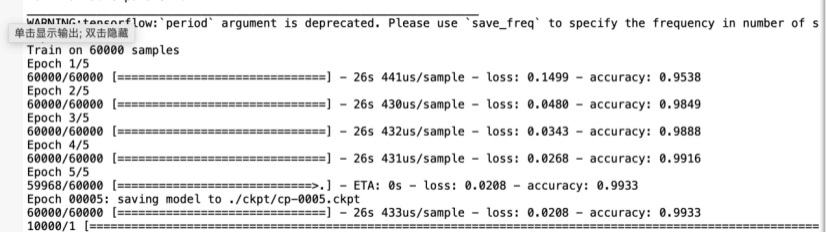
3.构建模型
class CNN(object):
    def __init__(self):
        model = models.Sequential()
        # 第1层卷积,卷积核大小为3*3,32个,28*28为待训练图片的大小
        model.add(layers.Conv2D(32, (3, 3), activation='relu', input_shape=(28, 28, 1)))
        model.add(layers.MaxPooling2D((2, 2)))
        # 第2层卷积,卷积核大小为3*3,64个
        model.add(layers.Conv2D(64, (3, 3), activation='relu'))
        model.add(layers.MaxPooling2D((2, 2)))
        # 第3层卷积,卷积核大小为3*3,64个
        model.add(layers.Conv2D(64, (3, 3), activation='relu'))

        model.add(layers.Flatten())
        model.add(layers.Dense(64, activation='relu'))
        model.add(layers.Dense(10, activation='softmax'))

        model.summary()
        self.model = model
4.编译训练模型
class Train:
def __init__(self):
self.cnn = CNN()
self.data = DataSource()
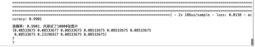
def train(self):
check_path = './ckpt/cp-{epoch:04d}.ckpt'
# period 每隔5epoch保存一次
save_model_cb = tf.keras.callbacks.ModelCheckpoint(check_path, save_weights_only=True, verbose=1, period=5)
self.cnn.model.compile(optimizer='adam',
loss='sparse_categorical_crossentropy',
metrics=['accuracy'])
self.cnn.model.fit(self.data.train_images, self.data.train_labels, epochs=5, callbacks=[save_model_cb])
test_loss, test_acc = self.cnn.model.evaluate(self.data.test_images, self.data.test_labels)
print("准确率: %.4f,共测试了%d张图片 " % (test_acc, len(self.data.test_labels)))
5.开启训练
if __name__ == "__main__":
    print(tf.__version__)
app = Train()
3.3.4结果展示


 7043
7043


 被折叠的 条评论
为什么被折叠?
被折叠的 条评论
为什么被折叠?
 到【灌水乐园】发言


