


目录
1.R语言介绍


2.R语言安装
CARN → 选择China中任意镜像站点 → Download R for Windows → base(二进制版本R基础软件)→
Download R-4.2.2 for Windows (76 megabytes, 64 bit)
3.Rstudio安装
https://posit.co/download/rstudio-desktop/
DOWNLOAD RSTUDIO → DOWNLOAD RSTUDIO DESKTOP FOR WINDOWS → RStudio
Desktop → DOWNLOAD RSTUDIO → DOWNLOAD RSTUDIO DESKTOP FOR WINDOWS
4.Rtoos安装(R包安装需要)
https://cran.r-project.org/bin/windows/Rtools/rtools43/rtools.html
→Rtools43 installer
5.基本操作
查看当前工作目录 :getwd()
设置工作目录 :setwd(dir = "路径")
注意:Rwindow语言路径使用’\’ 而R语言使用’/'
查看工作目录下的文件:list.files() 或者 dir()
查看帮助文档 :help.start();
函数详情 help(sum)
查看函数参数 args(函数名)
查看包帮助文档: help(package=包名vig)
> getwd()
[1] "C:/Users/xiaob/Desktop"
> setwd(dir = "C:/Users/xiaob/Desktop/Rwork")
> getwd()
[1] "C:/Users/xiaob/Desktop/Rwork"
> list.files()
character(0)
> dir()
character(0)
赋值符号 ‘<-’ (等号可以不推荐)
赋值给全局变量 ‘<<-’
> x<-2
> x
[1] 2
> x<<-5
> x
[1] 5
> z <- sum(1,2,3,4,5)
> z
[1] 15
> t <- min(1,2,3,4,5)
> t
[1] 1

> ls()  #查看所有变量
[1] "t" "x" "y" "z"
> ls.str() #查看所有变量和变量值
t :  num 1
x :  num 5
y :  num 4
z :  num 15
> str(x)
 num 5
> rm(x) #删除变量
> x
Error: object 'x' not found
> rm(t,y,z) #删除多个变量
> z
Error: object 'z' not found

> x<-2
> y<-4
> z<-8
> ls()
[1] "x" "y" "z"
> rm(list = ls())  #删除当前所有变量
> ls()
character(0)

上下移动光标选择命令
> history()  #查看历史命令
> history(5) #查看最近5条命令
清除命令窗口:ctrl + L
注释:#
保存工作空间:> save.image()
退出R: >q()
6.R包
(一)安装
查看包:https://cran.r-project.org/web/views/
1.在线安装
安装包:>install.packages() #需要选择镜像站点
安装指定包 :>install.packages("包名")
会自动安装依赖包
查看所有本地包安装路径:>libPaths()
查看所有已安装包列表:>library()
手动更改镜像:Tools → Global option → Packages
2.GitHub安装
GitHub搜索包名
> install.packages("devtools")
> install.packages("remotes")
> devtools::install_github("仓库名/包名")
3.本地安装
github仓库先下载压缩包
> devtools::install_local("绝对路径")
#注意改反斜杠
(二)使用
载入包: library(包名) 或者 require(包名)
查看包帮助文档 >help(package="包名")
查看包基本信息 >library(help="包名")
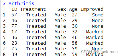
输入包内索引名可以直接查看数据集(注意需要先载入)
library(vcd)
library(help="vcd")

查看包内函数: ls("package:包名")
查看包内所有数据集 data(package="包名")
移除加载包: detach("package:包名")
查看当前已安装R包 installed.packages()
7.内置数据集
查看内置全部数据集 >help(package="datasets")
简略查看全部数据集 >data()
访问数据集:输入数据集名称
查看某个数据集详细信息:help("数据集名称")
8.数据结构
数据类型:


9.向量(集合)
1.基本操作
创建:>c(元素1,元素2,.....)
>x <- c(1,2,3,4)
>x
[1] 1 2 3 4

#逻辑型向量必须大写
> z <- c(TRUE,T,F)
> z
[1]  TRUE  TRUE FALSE
> z <- c(True,T,F)
Error: object 'True' not found

> c(1:20)  #生成1到20的等差数列
 [1]  1  2  3  4  5  6  7  8  9 10 11 12 13 14 15 16 17 18
[19] 19 20

> seq(from=1,to=100,by=2)  #生成步长为2的等差数列
 [1]  1  3  5  7  9 11 13 15 17 19 21 23 25 27 29 31 33 35
[19] 37 39 41 43 45 47 49 51 53 55 57 59 61 63 65 67 69 71
[37] 73 75 77 79 81 83 85 87 89 91 93 95 97 99

> seq(from=1,to=100,length.out=10)  #生成十个值的等差数列
 [1]   1  12  23  34  45  56  67  78  89 100

#向量化编程,批量计算
> x <- c(1,2,3,4,5)
> y <- c(6,7,8,9,10)
> x*2+y
[1]  8 11 14 17 20

> x[x>3]  #取出x中大于3的值
[1] 4 5
2.向量索引
R索引从1开始
> x <- c(1:10) #生成1到10的等差数列
> x
 [1]  1  2  3  4  5  6  7  8  9 10
> length(x)  #集合长度
[1] 10
> x[3]
[1] 3
> x[-9]  #不输出第9个元素
[1]  1  2  3  4  5  6  7  8 10

> x[c(2:6)]  #输出第2到第6个元素
[1] 2 3 4 5 6
> x[c(2,4,6)]  #输出2,4,6元素
[1] 2 4 6

> y <- c(1:5)
> y[c(T,F,T,T,F)]  #只输出逻辑为真的值
[1] 1 3 4

> y[y>2&y<5]
[1] 3 4

> v <- c(1:3)
> v
[1] 1 2 3
> v[c(4,5,6)] <- c(4,5,6)
> v
[1] 1 2 3 4 5 6
> v[20] <- 4
> v
 [1]  1  2  3  4  5  6 NA NA NA NA NA NA NA NA NA NA NA NA NA  4
插入向量
> v <- c(1:5)
> v
[1] 1 2 3 4 5
> append(x = v,values = 99,after = 2)  #在第二个元素后面插入99
[1]  1  2 99  3  4  5
rm(v) #删除整个向量
3.向量运算
> x <- 1:10
> x
 [1]  1  2  3  4  5  6  7  8  9 10
> x+1
 [1]  2  3  4  5  6  7  8  9 10 11
> x-3
 [1] -2 -1  0  1  2  3  4  5  6  7
> x <- x+1
> x
 [1]  2  3  4  5  6  7  8  9 10 11
> y <- seq(1,100,length.out = 10) #生成长度为10的等差数列
> y
 [1]   1  12  23  34  45  56  67  78  89 100
> x + y
 [1]   3  15  27  39  51  63  75  87  99 111
> x
 [1]  2  3  4  5  6  7  8  9 10 11
> y
 [1]   1  12  23  34  45  56  67  78  89 100
> x**y  #x的y次幂
 [1]  2.000000e+00  5.314410e+05  7.036874e+13
 [4]  5.820766e+23  1.039456e+35  2.115876e+47
 [7]  3.213876e+60  2.697216e+74  1.000000e+89
[10] 1.378061e+104
> y%%x #取余运算
 [1] 1 0 3 4 3 0 3 6 9 1
> y%/%x #整除运算
 [1] 0 4 5 6 7 8 8 8 8 9

#判断是否元素包含
> c(1,2,3) %in% c(1,2,2,4,5,6)
[1]  TRUE  TRUE FALSE
10.函数
> x <- -5:5
> x
 [1] -5 -4 -3 -2 -1  0  1  2  3  4  5
> abs(x)  #绝对值
 [1] 5 4 3 2 1 0 1 2 3 4 5
> sqrt(x) #开根号
 [1]      NaN      NaN      NaN      NaN      NaN 0.000000 1.000000 1.414214 1.732051 2.000000
[11] 2.236068
Warning message:
In sqrt(x) : NaNs produced
> sqrt(25) #开根号
[1] 5
> log(16,base=2)  #2为底 16的对数
[1] 4
> log(16)  #自然对数
[1] 2.772589

> exp(x)  #e的x次方
 [1] 6.737947e-03 1.831564e-02 4.978707e-02 1.353353e-01 3.678794e-01 1.000000e+00 2.718282e+00 7.389056e+00 2.008554e+01 5.459815e+01 1.484132e+02

#ceiling(a) 返回不小于a的最小整数
> ceiling(c(-2.3,3.1415))
[1] -2  4

#floor(x) 返回不大于x的最大整数
> floor(c(-2.3,3.1415))
[1] -3  3

#trunc(x) 返回整数部分
> trunc(c(-2.3,3.1415))
[1] -2  3

#roud(x,digits=保留小数位数) 对x四舍五入
> round(c(-2.3,3.1415))
[1] -2  3
> round(c(-2.3,3.1415),digits = 2)
[1] -2.30  3.14
#signif(x,digits=保留小数位数) 对x四舍五入  仅保留有效数字
> signif(c(-2.3,3.1415),digits=2)
[1] -2.3  3.1
> sin(x)
 [1]  0.9589243  0.7568025 -0.1411200 -0.9092974 -0.8414710  0.0000000  0.8414710  0.9092974
 [9]  0.1411200 -0.7568025 -0.9589243
> cos(x)
 [1]  0.2836622 -0.6536436 -0.9899925 -0.4161468  0.5403023  1.0000000  0.5403023 -0.4161468
 [9] -0.9899925 -0.6536436  0.2836622

> vec <- 1:10
> vec
 [1]  1  2  3  4  5  6  7  8  9 10
> sum(vec)
[1] 55
> max(vec)
[1] 10
> min(vec)
[1] 1
> range(vec) #返回最大值最小值
[1]  1 10
> var(vec)  #返回向量的方差
[1] 9.166667
11.矩阵与数组
矩阵
> m <- matrix(1:20,4,5)  #定义四行五列的数组
> m
     [,1] [,2] [,3] [,4] [,5]
[1,]    1    5    9   13   17
[2,]    2    6   10   14   18
[3,]    3    7   11   15   19
[4,]    4    8   12   16   20
> matrix(1:20,4,6)  #维数不对,报错
     [,1] [,2] [,3] [,4] [,5] [,6]
[1,]    1    5    9   13   17    1
[2,]    2    6   10   14   18    2
[3,]    3    7   11   15   19    3
[4,]    4    8   12   16   20    4
Warning message:
In matrix(1:20, 4, 6) :
  data length [20] is not a sub-multiple or multiple of the number of columns [6]
> m <- matrix(1:20,4)
> m
     [,1] [,2] [,3] [,4] [,5]
[1,]    1    5    9   13   17
[2,]    2    6   10   14   18
[3,]    3    7   11   15   19
[4,]    4    8   12   16   20
> m <- matrix(1:20,4,byrow = T)
> m
     [,1] [,2] [,3] [,4] [,5]
[1,]    1    2    3    4    5
[2,]    6    7    8    9   10
[3,]   11   12   13   14   15
[4,]   16   17   18   19   20
> m <- matrix(1:20,4,byrow = F)
> m
     [,1] [,2] [,3] [,4] [,5]
[1,]    1    5    9   13   17
[2,]    2    6   10   14   18
[3,]    3    7   11   15   19
[4,]    4    8   12   16   20
> rnames <- c("R1","R2","R3","R4")
> rnames
[1] "R1" "R2" "R3" "R4"
> cnames <- c("c1","c2","c3","c4","c5")
> cnames
[1] "c1" "c2" "c3" "c4" "c5"
> dimnames(m) <- list(rnames,cnames)
> m
   c1 c2 c3 c4 c5
R1  1  5  9 13 17
R2  2  6 10 14 18
R3  3  7 11 15 19
R4  4  8 12 16 20
数组
> x <- 1:20
> dim(x) <- c(2,2,5)
> x
, , 1

     [,1] [,2]
[1,]    1    3
[2,]    2    4

, , 2

     [,1] [,2]
[1,]    5    7
[2,]    6    8

, , 3

     [,1] [,2]
[1,]    9   11
[2,]   10   12

, , 4

     [,1] [,2]
[1,]   13   15
[2,]   14   16

, , 5

     [,1] [,2]
[1,]   17   19
[2,]   18   20
12.列表

> a <- 1:20
> b <- matrix(1:20,4)
> c <- mtcars
> d <- "This is a test list"
> mlist <- list(a,b,c,d)
> a <- 1
> b <- "saslkd"
> c <- 3.12
> #给列表指定key
> elist <- list(fist=a,second=b,third=c)
> elist[1]
$fist
[1] 1

> elist$fist
[1] 1

> class(elist[1])  #一个中括号还是列表
[1] "list"
> class(elist[[1]]) #两个中括号是数据本身
[1] "numeric"

> elist[[4]] = "sd"  #给列表赋值需要两个中括号
> elist
$fist
[1] 1

$second
[1] "saslkd"

$third
[1] 3.12

[[4]]
[1] "sd"
13.数据框


14.因子
15.获取数据
1.手动获取
> patientID <- c(1,2,3,4)
> admdate <- c("10/15/2009","11/01/2009","10/21/2009","10/29/2039")
> age <- c(25,34,28,52)
> diabetes <- c("Type1","Types","Type1","Type1")
> status <- c("Poor","Improved","Excellent","Poor")
> data <- data.frame(patientID,admdate,age,diabetes,status)
> data
  patientID    admdate age diabetes
1         1 10/15/2009  25    Type1
2         2 11/01/2009  34    Types
3         3 10/21/2009  28    Type1
4         4 10/29/2039  52    Type1
     status
1      Poor
2  Improved
3 Excellent
4      Poor
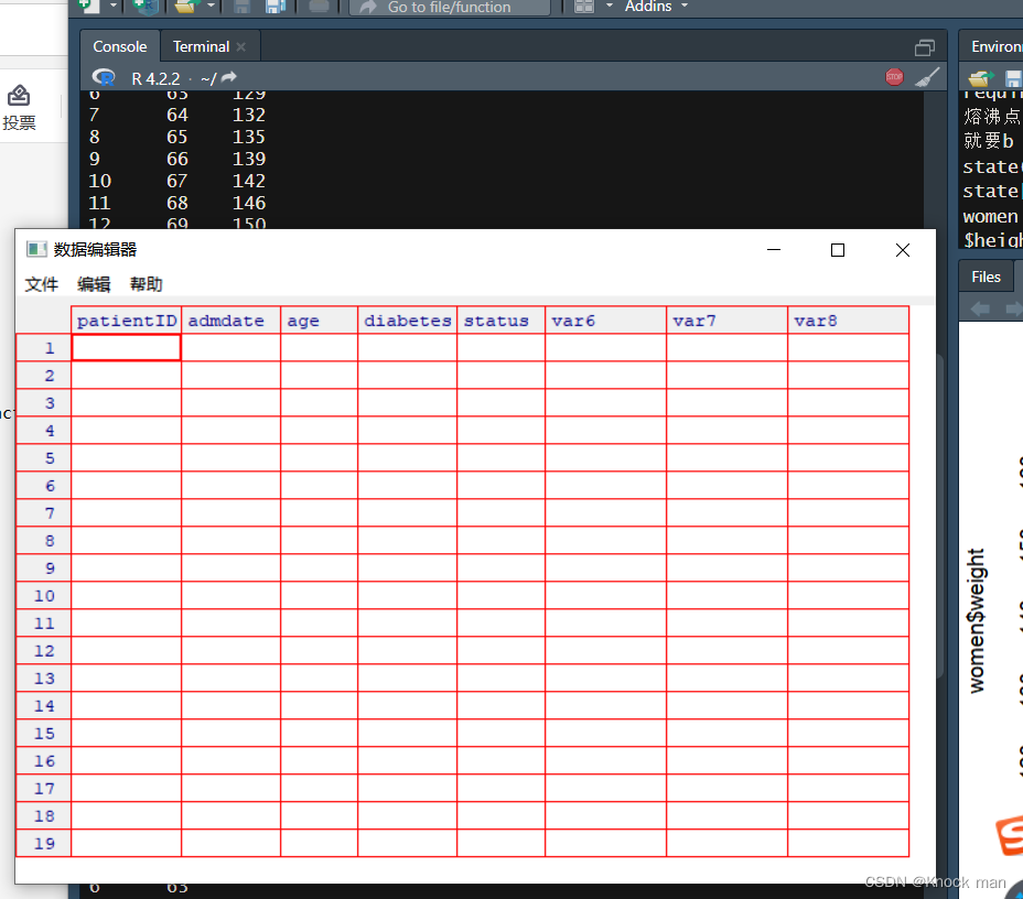
用键盘图形化输入数据
> patientID <- c(1,2,3,4)
> admdate <- c("10/15/2009","11/01/2009","10/21/2009","10/29/2039")
> age <- c(25,34,28,52)
> diabetes <- c("Type1","Types","Type1","Type1")
> status <- c("Poor","Improved","Excellent","Poor")
> data2 <- data.frame(patientID=character(0),admdate=character(0),age=numeric(),diabetes=character(),status=character())
> data2 <- edit(data2)   或者    fix(data2)
2.读取文件

读纯文本
使用
x <-read.table("路径",header=是否避开第一行,sep="分隔符",skip= 第几行开始,nrows = 第几行结束)
> x <- read.table("C:/Users/xiaob/Desktop/test.txt",sep=" ")
> x
  V1 V2 V3
1  a  b  c
2  1  2  3
3  4  5  6
4  7  8  9
5  2  3  4
6  5  6  7
7  8  9  5

> head(x,3)
  V1 V2 V3
1  a  b  c
2  1  2  3
3  4  5  6

> tail(x,2)
  V1 V2 V3
6  5  6  7
7  8  9  5
> x <- read.table("C:/Users/xiaob/Desktop/test.txt",header=TRUE,sep=" ",skip= 2,nrows = 5)
> x
  X4 X5 X6
1  7  8  9
2  2  3  4
3  5  6  7
4  8  9  5
5 12 45 67
3.写入文件
写入文本文件:
write.table(x,"C:/Users/xiaob/Desktop/test2.txt")
写入CSV文件:
write.csv(x,"C:/Users/xiaob/Desktop/test2.csv")
不写入序号列 设置row.names = FALSE
write.csv(x,"C:/Users/xiaob/Desktop/test2.csv",row.names = FALSE)
16.读取Excel格式文件
1.读取CSV文件
> x <- read.csv("C:/Users/xiaob/Desktop/test2.csv",header = TRUE)
> x
   V1 V2 V3
1   a  b  c
2   1  2  3
3   4  5  6
4   7  8 nu
5   2  3  4
6   5 nu  7
7   8  9  5
8  12 45 67
9  43 76 56
10 67 34 75
11 11 34 67
12 89 45 23
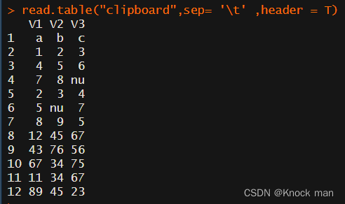
第二种方式,先复制到剪切板,然后跑一下代码
read.table("clipboard",sep= '\t' ,header = T)
2.读取XLS文件中的表格
install.packages("readxl")
library(readxl)
df <- read_excel("C:/Users/xiaob/Desktop/demo01.xls", sheet = "Sheet1")
view(df)
17.读取R文件
保存RDS文件
saveRDS(变量,file="文件名.RDS")
读取RDS文件
x <- readRDS("文件名")
> saveRDS(iris,file="iris.RDS")
> x = readRDS("C:/Users/xiaob/Desktop/Rwork/iris.RDS")
> x
    Sepal.Length Sepal.Width Petal.Length Petal.Width    Species
1            5.1         3.5          1.4         0.2     setosa
2            4.9         3.0          1.4         0.2     setosa
3            4.7         3.2          1.3         0.2     setosa
4            4.6         3.1          1.5         0.2     setosa
5            5.0         3.6          1.4         0.2     setosa
6            5.4         3.9          1.7         0.4     setosa
7            4.6         3.4          1.4         0.3     setosa
8            5.0         3.4          1.5         0.2     setosa
#保存指定对象
> save(iris,iris3,file = "C:/Users/xiaob/Desktop/Rwork/R2.RData")
#保存所有工作空间
> save.image()
18.线性回归
一元线性回归
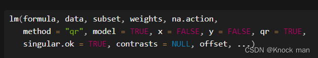
lm(解释变量 ~ 响应变量,数据集)
> fit <- lm(weight ~ height,data = women)
> summary.lm(fit)
#Call:公式  Residuals:残差
#Coefficients:系数项  Intercept:截距项
Call:
lm(formula = weight ~ height, data =women)
Residuals:
    Min      1Q  Median      3Q     Max
-1.7333 -1.1333 -0.3833  0.7417  3.1167

Coefficients:
             Estimate Std. Error t value Pr(>|t|)
(Intercept) -87.51667    5.93694  -14.74 1.71e-09 ***
height        3.45000    0.09114   37.85 1.09e-14 ***
---
Signif. codes:  0 ‘***’ 0.001 ‘**’ 0.01 ‘*’ 0.05 ‘.’ 0.1 ‘ ’ 1

Residual standard error: 1.525 on 13 degrees of freedom
Multiple R-squared:  0.991,	Adjusted R-squared:  0.9903
F-statistic:  1433 on 1 and 13 DF,  p-value: 1.091e-14

分析出公式为:weight = 3.45000(height   ) - 87.51667
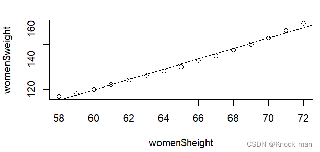
> plot(women$height,women$weight)  #画散点图
> abline(fit) #画直线
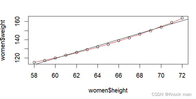
> fit2 <- lm(weight ~ height+I(height^2),data=women)
> fit2

Call:
lm(formula = weight ~ height + I(height ^2), data = women)

Coefficients:
  (Intercept)         height  I(height * 2)
       -87.52           3.45             NA

> summary(fit2)

Call:
lm(formula = weight ~ height + I(height * 2), data = women)

Residuals:
    Min      1Q  Median      3Q     Max
-1.7333 -1.1333 -0.3833  0.7417  3.1167

Coefficients: (1 not defined because of singularities)
               Estimate Std. Error t value Pr(>|t|)
(Intercept)   -87.51667    5.93694  -14.74 1.71e-09 ***
height          3.45000    0.09114   37.85 1.09e-14 ***
I(height * 2)        NA         NA      NA       NA
---
Signif. codes:  0 ‘***’ 0.001 ‘**’ 0.01 ‘*’ 0.05 ‘.’ 0.1 ‘ ’ 1

Residual standard error: 1.525 on 13 degrees of freedom
Multiple R-squared:  0.991,	Adjusted R-squared:  0.9903
F-statistic:  1433 on 1 and 13 DF,  p-value: 1.091e-14

> plot(women$height,women$weight)
> abline(fit) #画直线
>lines(women$height,fitted(fit2),col="red")  #画曲线
多元线性回归
state.x77
               Population Income Illiteracy Life Exp Murder HS Grad
Alabama              3615   3624        2.1    69.05   15.1    41.3
Alaska                365   6315        1.5    69.31   11.3    66.7
Arizona              2212   4530        1.8    70.55    7.8    58.1
Arkansas             2110   3378        1.9    70.66   10.1    39.9

#转为数据框存储
> states <- as.data.frame(state.x77,"Murder","Population","Illiteracy","Income","Frost")
> fit <- lm(Murder ~ Population+Illiteracy+Income+Frost,data = states)
> summary(fit)

Call:
lm(formula = Murder ~ Population + Illiteracy + Income + Frost,
    data = states)

Residuals:
    Min      1Q  Median      3Q     Max
-4.7960 -1.6495 -0.0811  1.4815  7.6210

Coefficients:
             Estimate Std. Error t value Pr(>|t|)
(Intercept) 1.235e+00  3.866e+00   0.319   0.7510
Population  2.237e-04  9.052e-05   2.471   0.0173 *
Illiteracy  4.143e+00  8.744e-01   4.738 2.19e-05 ***
Income      6.442e-05  6.837e-04   0.094   0.9253
Frost       5.813e-04  1.005e-02   0.058   0.9541
---
Signif. codes:  0 ‘***’ 0.001 ‘**’ 0.01 ‘*’ 0.05 ‘.’ 0.1 ‘ ’ 1

Residual standard error: 2.535 on 45 degrees of freedom
Multiple R-squared:  0.567,	Adjusted R-squared:  0.5285
F-statistic: 14.73 on 4 and 45 DF,  p-value: 9.133e-08

#查看方程参数
> coef(fit)
 (Intercept)   Population   Illiteracy       Income        Frost
1.2345634112 0.0002236754 4.1428365903 0.0000644247 0.0005813055
汽车数据集预测
mtcars
> fit <- lm(mpg ~ hp+wt+hp:wt,data = mtcars)  #hp与wt有某种交互关系
> summary(fit)


 2万+
2万+


 被折叠的 条评论
为什么被折叠?
被折叠的 条评论
为什么被折叠?
 到【灌水乐园】发言


