


广义线性模型已经不再局限于各个变量之间得服从正态分布和连续性变量要求;
其主要采用最大似然估计法进行系数计算,可应用于非常多的特定场景。
常用的有两个:
- logistics回归----解决通过一系列连续性或类别型变量来预测二值结果变量;
- Posion回归-------解决通过一系列连续性或类别型变量来预测计数型结果变量;
我们将通过AER包的Affair数据集(国外婚外情调查数据)来探究是哪些具体的、重要的因素会让人产生婚外情,
以及婚姻评分对婚外情的影响。
1、数据探索
#affair=婚外情事件次数
#gender=性别;female:男性;male:女性
#yearmarried=结婚年份
#religiousness=宗教信仰
#occuption=职业
#rating=婚姻评价

data(Affairs,package = "AER")
summary(Affairs)
par(mfrow=c(3,3))
name<-names(Affairs)
for (i in 1:9) {
           plot(table(Affairs[,i]),type = "b",main=name[i])
}


> summary(Affairs)
    affairs          gender         age         yearsmarried    children  religiousness
Min.   : 0.000   female:315   Min.   :17.50   Min.   : 0.125   no :171   Min.   :1.000
1st Qu.: 0.000   male  :286   1st Qu.:27.00   1st Qu.: 4.000   yes:430   1st Qu.:2.000
Median : 0.000                Median :32.00   Median : 7.000             Median :3.000
Mean   : 1.456                Mean   :32.49   Mean   : 8.178             Mean   :3.116
3rd Qu.: 0.000                3rd Qu.:37.00   3rd Qu.:15.000             3rd Qu.:4.000
Max.   :12.000                Max.   :57.00   Max.   :15.000             Max.   :5.000
   education       occupation        rating
Min.   : 9.00   Min.   :1.000   Min.   :1.000
1st Qu.:14.00   1st Qu.:3.000   1st Qu.:3.000
Median :16.00   Median :5.000   Median :4.000
Mean   :16.17   Mean   :4.195   Mean   :3.932
3rd Qu.:18.00   3rd Qu.:6.000   3rd Qu.:5.000
Max.   :20.00   Max.   :7.000   Max.   :5.000
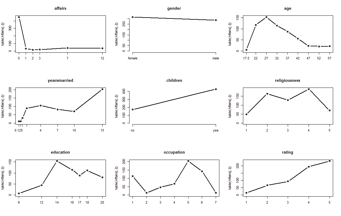
通过数据探索,得到每个数的5个基本统计指标和频数可视化我们得到如下简要结论:
- affair的婚外偷腥次数最多达到了12次,最小值为0次,并且0次居多,也就是说大部分人(72%)是不进行婚外情的。
- gender中男女比例从数值和图示来看基本一致男(47%);
- age代表被调查者的年龄分布来看在区间22-37岁年龄段调查者居多,样本年龄中位数为32岁;
- yearsmarried表示结婚年限,15年的老夫妻竟然很多!其他年龄段相对较均匀;
- children结合具体数值来看有72%的人有孩子;
- ...
2、数据处理
Affairs$ynaffair[Affairs$affairs>0]<-1
Affairs$ynaffair[Affairs$affairs==0]<-0
Affairs$ynaffair<-factor(Affairs$ynaffair,
                         levels = c(0,1),
                         labels = c("NO","YES"))
table(Affairs$ynaffair)
head(Affairs)

> table(Affairs$ynaffair)

NO YES
451 150
> head(Affairs)
   affairs gender age yearsmarried children religiousness education occupation rating ynaffair
4        0   male  37        10.00       no             3        18          7      4       NO
5        0 female  27         4.00       no             4        14          6      4       NO
11       0 female  32        15.00      yes             1        12          1      4       NO
16       0   male  57        15.00      yes             5        18          6      5       NO
23       0   male  22         0.75       no             2        17          6      3       NO
29       0 female  32         1.50       no             2        17          5      5       NO
3、logisic回归
#logisic回归
fit.full<-glm(ynaffair~gender+age+yearsmarried+children+
                religiousness+education+occupation+rating,
              data = Affairs,
              family = binomial(link = "logit"))
summary(fit.full)
#逐步回归
glm.full<-step(fit.full)
summary(glm.full)
#两者回归比较(变量选择评价)
anova(fit.full,glm.full,test = "Chisq")
#对逐步回归结果系数解释
coef(glm.full)#对数优势比
exp(coef(glm.full))#优势比


logisitc回归结果
> summary(fit.full)

Call:
glm(formula = ynaffair ~ gender + age + yearsmarried + children +
    religiousness + education + occupation + rating, family = binomial(link = "logit"),
    data = Affairs)

Deviance Residuals:
    Min       1Q   Median       3Q      Max
-1.5713  -0.7499  -0.5690  -0.2539   2.5191

Coefficients:
              Estimate Std. Error z value Pr(>|z|)
(Intercept)    1.37726    0.88776   1.551 0.120807
gendermale     0.28029    0.23909   1.172 0.241083
age           -0.04426    0.01825  -2.425 0.015301 *
yearsmarried   0.09477    0.03221   2.942 0.003262 **
childrenyes    0.39767    0.29151   1.364 0.172508
religiousness -0.32472    0.08975  -3.618 0.000297 ***
education      0.02105    0.05051   0.417 0.676851
occupation     0.03092    0.07178   0.431 0.666630
rating        -0.46845    0.09091  -5.153 2.56e-07 ***
---
Signif. codes:  0 ‘***’ 0.001 ‘**’ 0.01 ‘*’ 0.05 ‘.’ 0.1 ‘ ’ 1

(Dispersion parameter for binomial family taken to be 1)

    Null deviance: 675.38  on 600  degrees of freedom
Residual deviance: 609.51  on 592  degrees of freedom
AIC: 627.51

Number of Fisher Scoring iterations: 4

#逐步回归过程
> glm.full<-step(fit.full)
Start:  AIC=627.51
ynaffair ~ gender + age + yearsmarried + children + religiousness +
    education + occupation + rating

                Df Deviance    AIC
- education      1   609.68 625.68
- occupation     1   609.70 625.70
- gender         1   610.89 626.89
..............
Step:  AIC=623.86
ynaffair ~ gender + age + yearsmarried + religiousness + rating

                Df Deviance    AIC
<none>               611.86 623.86
- gender         1   615.36 625.36
- age            1   618.05 628.05
- religiousness  1   625.57 635.57
- yearsmarried   1   626.23 636.23
- rating         1   639.93 649.93

#逐步回归结果
> summary(glm.full)#逐步回归

Call:
glm(formula = ynaffair ~ gender + age + yearsmarried + religiousness +
    rating, family = binomial(link = "logit"), data = Affairs)

Deviance Residuals:
    Min       1Q   Median       3Q      Max
-1.5623  -0.7495  -0.5664  -0.2671   2.3975

Coefficients:
              Estimate Std. Error z value Pr(>|z|)
(Intercept)    1.94760    0.61234   3.181 0.001470 **
gendermale     0.38612    0.20703   1.865 0.062171 .
age           -0.04393    0.01806  -2.432 0.015011 *
yearsmarried   0.11133    0.02983   3.732 0.000190 ***
religiousness -0.32714    0.08947  -3.656 0.000256 ***
rating        -0.46721    0.08928  -5.233 1.67e-07 ***
---
Signif. codes:  0 ‘***’ 0.001 ‘**’ 0.01 ‘*’ 0.05 ‘.’ 0.1 ‘ ’ 1

(Dispersion parameter for binomial family taken to be 1)

    Null deviance: 675.38  on 600  degrees of freedom
Residual deviance: 611.86  on 595  degrees of freedom
AIC: 623.86

Number of Fisher Scoring iterations: 4

#两者回归方式进行检验
> anova(fit.full,glm.full,test = "Chisq")
Analysis of Deviance Table

Model 1: ynaffair ~ gender + age + yearsmarried + children + religiousness +
    education + occupation + rating
Model 2: ynaffair ~ gender + age + yearsmarried + religiousness + rating
  Resid. Df Resid. Dev Df Deviance Pr(>Chi)
1       592     609.51
2       595     611.86 -3  -2.3486   0.5033
4、增强系数解释(概率)与预测(新样本)
#由于采用书本知识原因,不采用逐步回归方法进行预测;(判断方法和之前基本一致)
#采用第一次回归的系数最显著地4个指标进行logistics回归
fit.reduce<-glm(ynaffair~rating+age+yearsmarried+religiousness,
                data = Affairs,family = binomial())
summary(fit.reduce)
anova(fit.reduce,fit.full,test = "Chisq")


#新数据集(探究婚姻满意度对婚外情的影响)
testdata<-data.frame(rating=c(1,2,3,4,5),
                     age=mean(Affairs$age),
                     yearsmarried=mean(Affairs$yearsmarried),
                     religiousness=mean(Affairs$religiousness))
testdata
testdata$prob<-predict(fit.reduce,newdata = testdata,type = "response")
testdata

#新数据集2(探究不同年龄对婚外情的影响)
testdata2<-data.frame(rating=mean(Affairs$rating),
                     age=seq(17,57,10),
                     yearsmarried=mean(Affairs$yearsmarried),
                     religiousness=mean(Affairs$religiousness))
testdata2
testdata2$prob2<-predict(fit.reduce,newdata = testdata,type = "response")
testdata2


> testdata
  rating      age yearsmarried religiousness      prob
1      1 32.48752     8.177696      3.116473 0.5302296
2      2 32.48752     8.177696      3.116473 0.4157377
3      3 32.48752     8.177696      3.116473 0.3096712
4      4 32.48752     8.177696      3.116473 0.2204547
5      5 32.48752     8.177696      3.116473 0.1513079

> testdata2
   rating age yearsmarried religiousness     prob2
1 3.93178  17     8.177696      3.116473 0.5302296
2 3.93178  27     8.177696      3.116473 0.4157377
3 3.93178  37     8.177696      3.116473 0.3096712
4 3.93178  47     8.177696      3.116473 0.2204547
5 3.93178  57     8.177696      3.116473 0.1513079
5、结果可视化
par(mfrow=c(1,2))
plot(testdata2$prob,type = "b",
     xlab = "rating",ylab = "prob",main = "婚姻满意度对婚外情影响",
     cex=3,lty=13,lwd=3,col=rainbow(5),pch=19,
     cex.lab=1.3,cex.axis=1.3,cex.main=1.5,)
plot(testdata2$prob2,type = "b",
     xlab = "age",ylab = "prob",main = "不同年龄段婚外情概率",
     cex=3,lty=18,lwd=3,col=rainbow(5),pch=17,
     cex.lab=1.3,cex.axis=1.3,cex.main=1.5,)

结论:控制其他因素影响,在相同条件下,rating(婚姻满意度)越高,婚外情的概率越低;
age(年龄)越高,婚外情的概率越低;
6、回归检验
过度离势会造成奇异的标准误检验和不精确的显著性检验,使得p值等失效,失去回归的可信度,因此要对回归进行过度离势检验。
> deviance(fit.reduce)/df.residual(fit.reduce)
[1] 1.03248
过度离势接近1,表明没有过度离势,P值和标准误检验有效。
附录
1、系数的优势比方面解释较为困难,可参考网址
(3)对一般Logistic模型系数的解释 - 简书
#由于p值没有通过,因此采用逐步回归结果进行系数解释
> coef(glm.full)#对数优势比
  (Intercept)    gendermale           age  yearsmarried
   1.94760307    0.38612217   -0.04392545    0.11132715
religiousness        rating
  -0.32714238   -0.46721157
> exp(coef(glm.full))#优势比
  (Intercept)    gendermale           age  yearsmarried
    7.0118605     1.4712644     0.9570253     1.1177605
religiousness        rating
    0.7209811     0.6267475
2、chi-square test)或称卡方检验,是一种用途较广的假设检验方法。可以分为成组比较(不配对资料)和个别比较(配对,或同一对象两种处理的比较)两类。
此处用来进行同一结果的两种回归进行比较,如果卡方检验通过了,表明两者回归本质是一样的,如果没有通过,那么两个回归就是不一样的,也就是说,通过逐步回归得到的(较少变量拟合)结果方式完全不一样,取得的效果确实更好的,因此可以采用后者方法进行解释。
借用一下王老板的Q版表情包~--------------蔡磊---原创笔记 2018-11-25


 1万+
1万+


 被折叠的 条评论
为什么被折叠?
被折叠的 条评论
为什么被折叠?
 到【灌水乐园】发言


