


本文使用streamlit为我上一个项目(据用户的社交媒体使用情况判断用户情绪 )为例做一个前端,我将详细讲解每个部分。本项目完全开源 百度网盘下载地址,夸克网盘下载地址,github
吐槽部分:我要讲一个学html没学会,结果发现streamlit居然这么好用的故事。本来我打算给我上一个通过用户社交媒体的使用情况预测情绪的项目写一个前端页面,可是我从来没有学过前端,于是决定从零开始学习html。可是不学不知道啊,这html可是人能写的???什么<head>,什么<style>,什么<h1><script>,简直没有一点可读性。。。
但是随后想想,毕竟学习是个痛苦的事情,算了吧,学不会是自己的问题,于是继续学,继续写。最后拼尽全力写出来了下图,可以通过用户输入的数据预测情绪(代码放在最后,本文重点讲streamlit)。
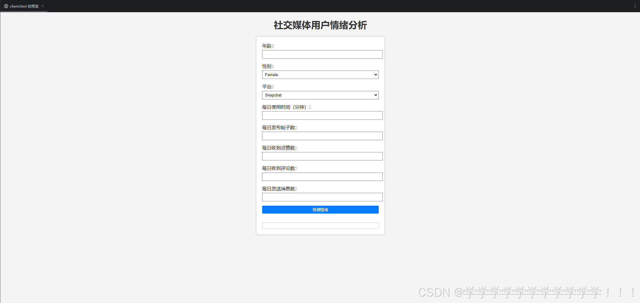
然后我们老师说可以用streamlit写一个简单的前端,我便尝试了一下,才发现原来还有这么爽的方法!话不多说,上成品!
上图是一小部分,下面我将一步一步来解释整个流程,全部的代码再最后
1.准备工作
1.1导包
import streamlit as st
# 导入pandas 和 numpy 用这两个库进行数据处理
import pandas as pd
import numpy as np
import time
# 用sns画图,看看最开始的数据长什么样
import matplotlib as mpl
import seaborn as sns  # Statistical data visualization
from sklearn.decomposition import PCA


# 决策树
from sklearn.metrics import confusion_matrix

from sklearn.tree import DecisionTreeClassifier
from sklearn.tree import export_graphviz
import graphviz
# k-nn(k-近邻)
from sklearn.neighbors import KNeighborsClassifier
# 支持向量机
from sklearn.svm import SVC
# 集成学习
from sklearn.ensemble import BaggingClassifier
# 保存模型
import joblib

# 各种评价标准
from sklearn.metrics import accuracy_score
from sklearn.metrics import precision_score
from sklearn.metrics import recall_score
from sklearn.metrics import f1_score

# 用来画图比较
import matplotlib.pyplot as plt
2.1读取数据集
# 将plt画出来的图设置为中文简体
mpl.rcParams['font.family'] = 'SimHei'

# 读取数据集
test_x = pd.read_csv(r"D:\social-media-usage-and-emotional-well-being\pythonProject\Data preprocessing\test_x.csv")
test_y = pd.read_csv(r"D:\social-media-usage-and-emotional-well-being\pythonProject\Data preprocessing\test_y.csv")
train_y = pd.read_csv(r"D:\social-media-usage-and-emotional-well-being\pythonProject\Data preprocessing\train_y.csv")
train_x = pd.read_csv(r"D:\social-media-usage-and-emotional-well-being\pythonProject\Data preprocessing\train_x.csv")
2.主要框架编写
2.1大框架
st.header("根据社交媒体使用情况判断用户情绪")

choice = st.sidebar.selectbox(
    label='请选择您想进行的操作',
    options=('预测情绪', '调试模型'),
    index=0,
    format_func=str,
)

if choice == '调试模型':
    pass
elif choice == '预测模型':
    pass
我们的大框架是想让用户自己选择,可以自己调试模型,也可以自己预测,所以首先把这两个选项写好
st.header("根据社交媒体使用情况判断用户情绪")是写一个大标题,choice=st.sidebar.selectbox(
是在侧边栏放一个选项框。现在的运行结果是这样的(通过在终端运行“streamlit run 文件名”)

接下来开始写调试模型的具体内容
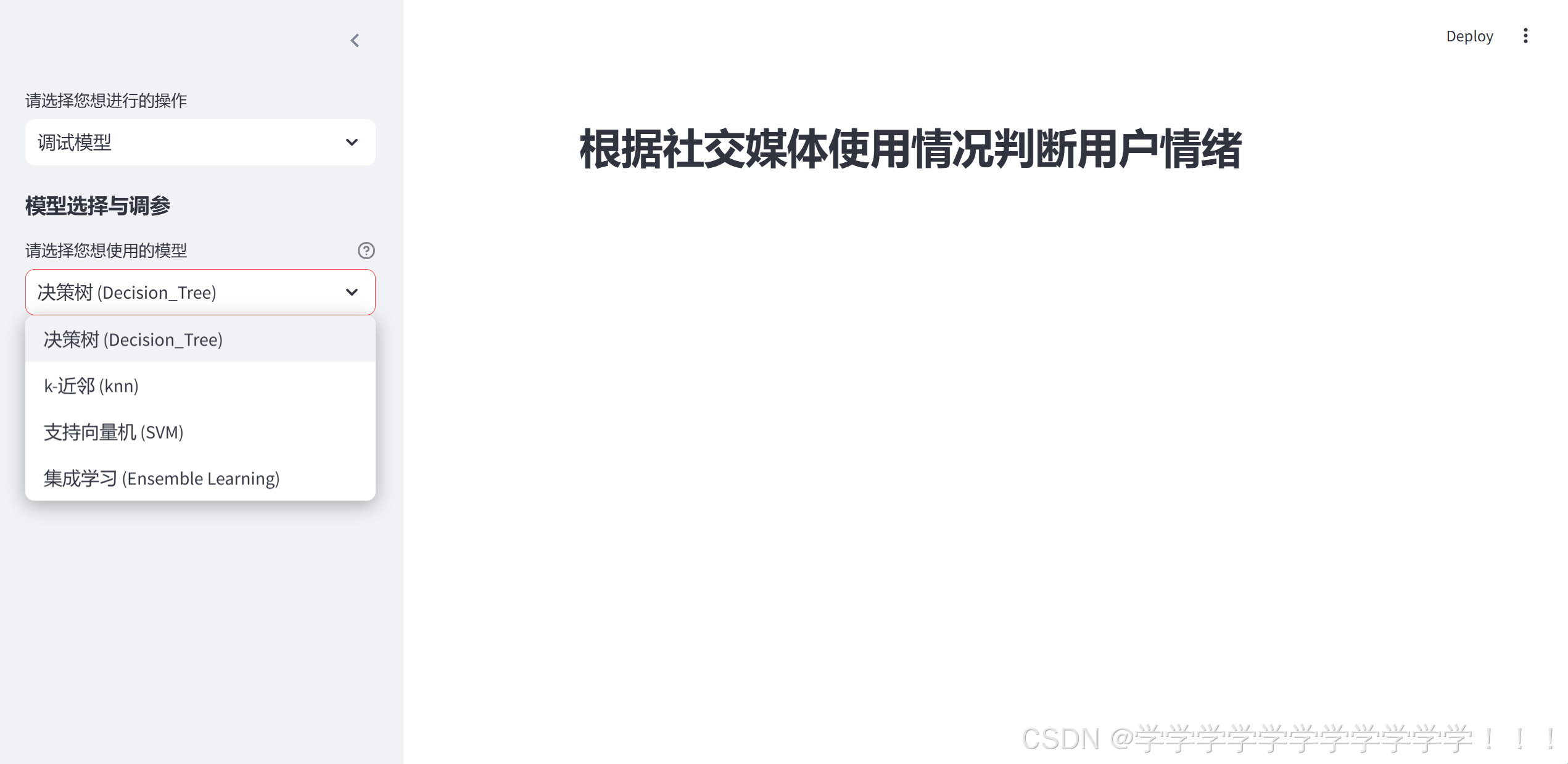
2.2调试模型部分
这里我们提供4种模型,分别是决策树,k-近邻,支持向量机,集成学习,贝叶斯因为准确率不高就没有加上。
if choice == '调试模型':
    st.sidebar.subheader('模型选择与调参')
    model = st.sidebar.selectbox(
        label='请选择您想使用的模型',
        options=('决策树 (Decision_Tree)', 'k-近邻 (knn)', '支持向量机 (SVM)', '集成学习 (Ensemble Learning)'),
        index=0,
        format_func=str,
        help='目前只提供这四种模型'
    )
    if model == '决策树 (Decision_Tree)':
        pass
    elif model == 'k-近邻 (knn)':
        pass
    elif model == '支持向量机 (SVM)':
        pass
    elif model == '集成学习 (Ensemble Learning)':
        pass
同样的,先在侧边栏加一个选项,可以选择想调试的模型,再一一对模型进行操作,现在的运行结果是这样的
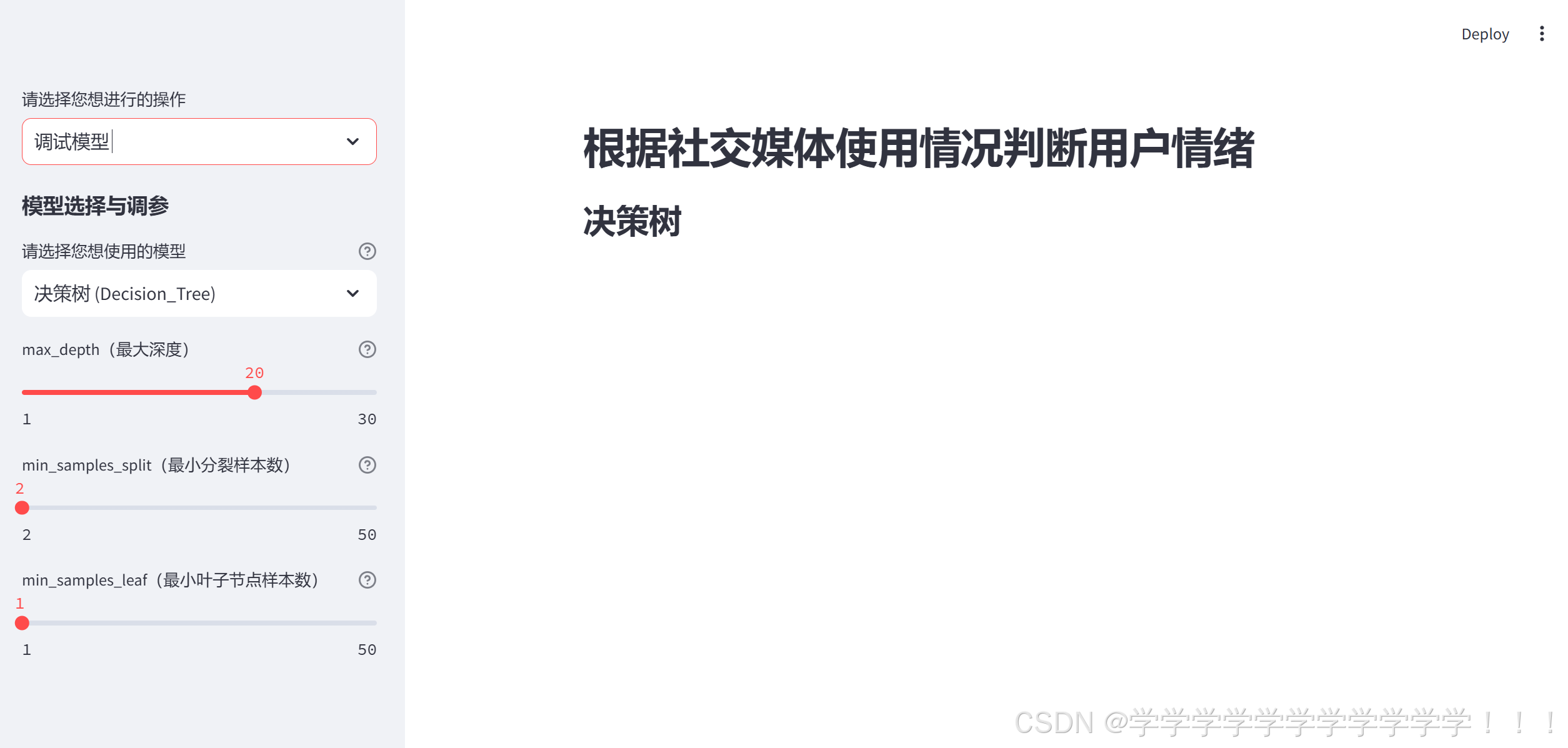
2.2.1决策树部分选项编写
    if model == '决策树 (Decision_Tree)':
        st.subheader('决策树')
        iterations = st.sidebar.slider("max_depth(最大深度)", 1, 30, 20, 1,
                                       help='决策树的最大深度,限制树的生长,防止过拟合.')
        min_samples_split1 = st.sidebar.slider("min_samples_split(最小分裂样本数)", 2, 50, 2, 1,
                                               help='内部节点再划分所需的最小样本数。')
        min_samples_leaf1 = st.sidebar.slider("min_samples_leaf(最小叶子节点样本数)", 1, 50, 1, 1,
                                              help='叶节点所需的最小样本数。')
这里的最大深度,最小分裂样本数,最小叶子节点样本数是对决策树模型调参用的
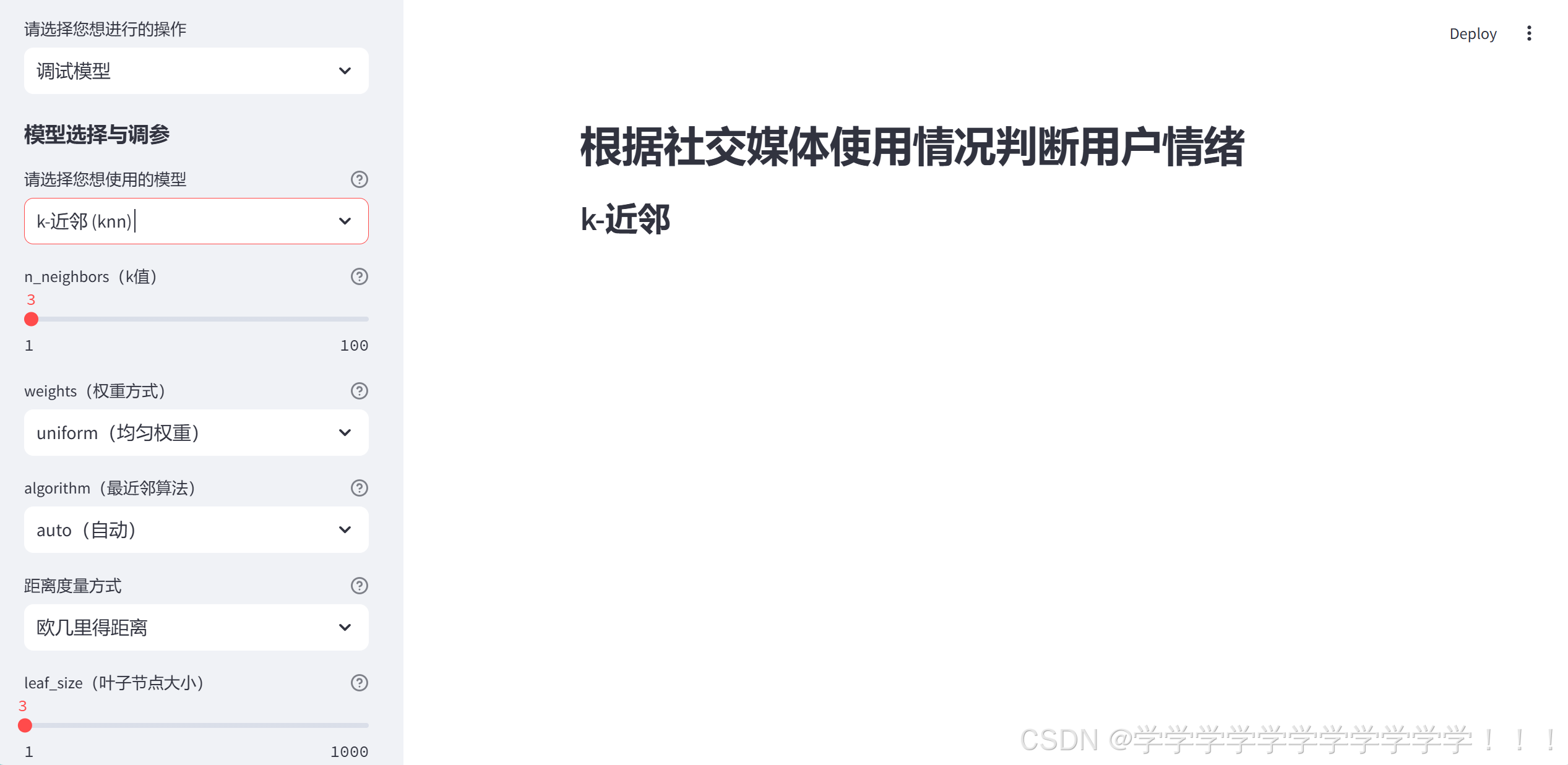
2.2.2k近邻部分选项编写
    elif model == 'k-近邻 (knn)':
        st.subheader('k-近邻')
        n_neighbors = st.sidebar.slider("n_neighbors(k值)", 1, 100, 3, 1,
                                       help='决策树的最大深度,限制树的生长,防止过拟合.')

        weights1 = st.sidebar.selectbox(
            label='weights(权重方式)',
            options=('uniform(均匀权重)', 'distance(距离加权)'),
            index=0,
            format_func=str,
            help='用于指定近邻样本的权重计算方式。'
        )
        if weights1 == 'uniform(均匀权重)':
            weights2 = 'uniform'
        else:
            weights2 = 'distance'

        algorithm1 = st.sidebar.selectbox(
            label='algorithm(最近邻算法)',
            options=('auto(自动)', 'ball_tree', 'kd_tree'),
            index=0,
            format_func=str,
            help='用于指定计算最近邻居的算法'
        )
        if algorithm1 == 'auto(自动)':
            algorithm1 = 'auto'

        p1 = st.sidebar.selectbox(
            label='距离度量方式',
            options=('欧几里得距离', '曼哈顿距离'),
            index=0,
            format_func=str,
            help='用于闵可夫斯基距离(metric = "minkowski")的参数。当p = 1时,闵可夫斯基距离就是曼哈顿距离;当p = 2时,就是欧几里得距离。。'
        )
        if p1 == '曼哈顿距离':
            p2 = 1
        else:
            p2 = 2

        leaf_size1 = st.sidebar.slider("leaf_size(叶子节点大小)", 1, 1000, 3, 1, help='这主要是用于 “ball_tree” 和 “kd_tree” 算法中的一个参数,它控制树的叶子节点大小。')
        progress_bar = st.empty()
设置各种参数,但是要把参数转化为sklearn可以接受的形式如
if weights1 == 'uniform(均匀权重)':
weights2 = 'uniform'
else:
weights2 = 'distance'
这部分就去掉了“(均匀权重)”,使得weights1直接可以传入sklearn的函数中,现在的运行结果是这样的
2.2.3支持向量机部分选项编写
    elif model == '支持向量机 (SVM)':
        st.subheader('支持向量机')

        kernel = st.sidebar.selectbox(
            label='kernel(核函数类型)',
            options=('rbf(径向基函数核)', 'linear(线性核)', 'polynomial(多项式核)'),
            index=0,
            format_func=str,
            help='核函数类型'
        )
        if kernel == 'rbf(径向基函数核)':
            kernel = 'rbf'
            c = st.sidebar.slider("C(惩罚参数)", 1, 10000, 10000, 1,
                                  help='控制对错误分类的惩罚程度')

        elif kernel == 'linear(线性核)':
            kernel = 'linear'
            c = st.sidebar.slider("C(惩罚参数)", 1, 10, 1, 1,
                                  help='控制对错误分类的惩罚程度')

        else:
            kernel = 'poly'
            c = st.sidebar.slider("C(惩罚参数)", 1, 1000, 100, 1,
                                  help='控制对错误分类的惩罚程度')

        shrinking = st.sidebar.selectbox(
            label='shrinking(是否使用收缩启发式)',
            options=(True, False),
            index=0,
            format_func=str,
            help='在训练过程中可能会改变优化算法的行为,不使用收缩启发式可能会使训练时间变长,但在某些特定情况下可能会提高模型的稳定性或者准确性。'
        )

        probability = st.sidebar.selectbox(
            label='probability(是否启用概率估计)',
            options=(True, False),
            index=0,
            format_func=str,
            help='在训练过程中可能会改变优化算法的行为,不使用收缩启发式可能会使训练时间变长,但在某些特定情况下可能会提高模型的稳定性或者准确性。'
        )
这里大家自己测试线性核和多项式核时运行会比较缓慢因为这两核会有比较大的计算量,现在的运行效果是这样的
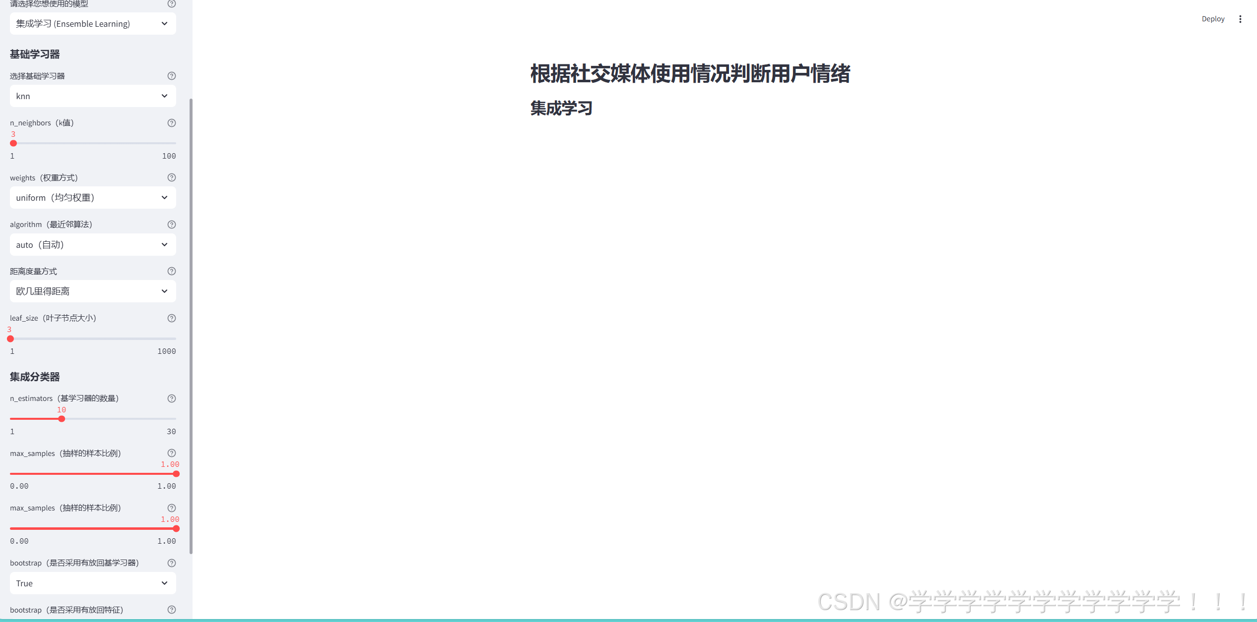
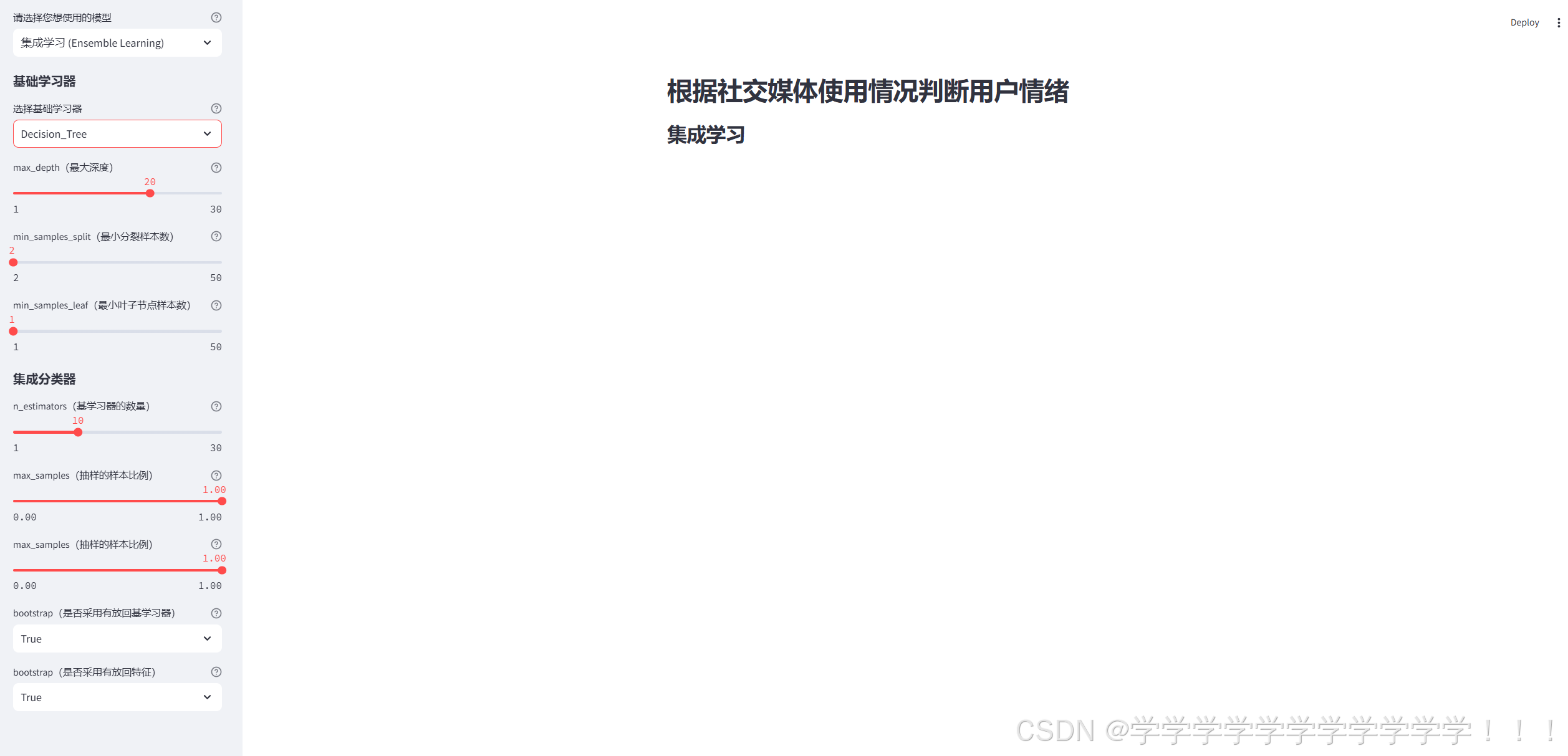
2.2.4集成学习部分选项编写
    elif model == '集成学习 (Ensemble Learning)':

        st.subheader("集成学习")
        st.sidebar.subheader('基础学习器')
        base_model = st.sidebar.selectbox(
            label='选择基础学习器',
            options=('Decision_Tree', 'knn'),
            index=0,
            format_func=str,
            help='在训练过程中可能会改变优化算法的行为,不使用收缩启发式可能会使训练时间变长,但在某些特定情况下可能会提高模型的稳定性或者准确性。'
        )


        #决策树
        if base_model=="Decision_Tree":
            iterations = st.sidebar.slider("max_depth(最大深度)", 1, 30, 20, 1,
                                           help='决策树的最大深度,限制树的生长,防止过拟合.')
            min_samples_split1 = st.sidebar.slider("min_samples_split(最小分裂样本数)", 2, 50, 2, 1,
                                                   help='内部节点再划分所需的最小样本数。')
            min_samples_leaf1 = st.sidebar.slider("min_samples_leaf(最小叶子节点样本数)", 1, 50, 1, 1,
                                                  help='叶节点所需的最小样本数。')


        else:
            n_neighbors = st.sidebar.slider("n_neighbors(k值)", 1, 100, 3, 1,
                                            help='决策树的最大深度,限制树的生长,防止过拟合.')

            weights1 = st.sidebar.selectbox(
                label='weights(权重方式)',
                options=('uniform(均匀权重)', 'distance(距离加权)'),
                index=0,
                format_func=str,
                help='用于指定近邻样本的权重计算方式。'
            )
            if weights1 == 'uniform(均匀权重)':
                weights2 = 'uniform'
            else:
                weights2 = 'distance'

            algorithm1 = st.sidebar.selectbox(
                label='algorithm(最近邻算法)',
                options=('auto(自动)', 'ball_tree', 'kd_tree'),
                index=0,
                format_func=str,
                help='用于指定计算最近邻居的算法'
            )
            if algorithm1 == 'auto(自动)':
                algorithm1 = 'auto'

            p1 = st.sidebar.selectbox(
                label='距离度量方式',
                options=('欧几里得距离', '曼哈顿距离'),
                index=0,
                format_func=str,
                help='用于闵可夫斯基距离(metric = "minkowski")的参数。当p = 1时,闵可夫斯基距离就是曼哈顿距离;当p = 2时,就是欧几里得距离。。'
            )
            if p1 == '曼哈顿距离':
                p2 = 1
            else:
                p2 = 2

            leaf_size1 = st.sidebar.slider("leaf_size(叶子节点大小)", 1, 1000, 3, 1,
                                           help='这主要是用于 “ball_tree” 和 “kd_tree” 算法中的一个参数,它控制树的叶子节点大小。')


        st.sidebar.subheader('集成分类器')
        n_estimators = st.sidebar.slider("n_estimators(基学习器的数量)", 1, 30, 10, 1,
                                       help='这个参数是可以调整的重要参数。它决定了集成学习中基学习器(例如决策树)的数量。增加n_estimators通常可以提高模型的性能和稳定性,但也会增加计算成本和训练时间。例如,当处理一个复杂的分类问题,数据有较多的噪声和特征时,适当增加n_estimators可能会使模型更好地拟合数据。')
        max_samples = st.sidebar.slider("max_samples(抽样的样本比例)", 0.0, 1.0, 1.0, format="%.2f",
                                       help='用于控制每次构建基学习器时从训练数据集中抽样的样本比例(如果值小于 1.0)或样本数量(如果值为整数)。调整这个参数可以改变基学习器训练数据的多样性。如果数据量很大,适当减小max_samples可以减少每个基学习器的训练时间,同时增加基学习器之间的差异。')
        max_features = st.sidebar.slider("max_samples(抽样的样本比例)", 0.0, 1.0, 1.0, format="%.2f",
                                       help='控制每次构建基学习器时从特征集合中抽取的特征比例(如果值小于 1.0)或特征数量(如果值为整数)。通过调整这个参数可以引入特征的随机性,特别是在特征维度较高的情况下,能够防止模型过度依赖某些特征,提高模型的泛化能力。')
        bootstrap = st.sidebar.selectbox(
            label='bootstrap(是否采用有放回基学习器)',
            options=(True, False),
            index=0,
            format_func=str,
            help='在训练过程中可能会改变优化算法的行为,不使用收缩启发式可能会使训练时间变长,但在某些特定情况下可能会提高模型的稳定性或者准确性。'
        )
        bootstrap_features = st.sidebar.selectbox(
            label='bootstrap(是否采用有放回特征)',
            options=(True, False),
            index=0,
            format_func=str,
            help='在训练过程中可能会改变优化算法的行为,不使用收缩启发式可能会使训练时间变长,但在某些特定情况下可能会提高模型的稳定性或者准确性。'
        )
这里需要注意的是因为集成学习需要基础学习器,这里的基础学习器提供了两个,分别是决策树和knn,所以要多谢两个选项,其实也不麻烦,直接把上面的全部复制粘贴就行。
现在的界面是这样的
现在我们把所有的选项和框架都编写好了,可以开始写具体功能实现了
3.具体功能实现
3.1决策树
        progress_bar = st.empty()

        with st.spinner('加载中...'):
            time.sleep(0.5)
            # 实例决策树
            Decision_Tree = DecisionTreeClassifier(criterion='entropy', max_depth=iterations, min_samples_split=min_samples_split1, min_samples_leaf=min_samples_leaf1, random_state=2024)
            # 训练决策树
            Decision_Tree.fit(train_x, train_y)
            joblib.dump(Decision_Tree,
                        'D:\social-media-usage-and-emotional-well-being\pythonProject\models\Decision_Tree_model.pickle')
            # 预测
这里添加time.sleep(0.5)是为了让看起来更加丝滑,有一个0.5秒的加载过程,而不是直接生硬的把结果输出,要注意的是再调用DecisionTreeClassifier函数的时候不要把参数写错搞混。jiblib.dump()函数是保存模型方便后来使用
# 预测
Decision_Tree_pred = Decision_Tree.predict(test_x)
# precision成绩
Decision_Tree_precision = precision_score(test_y, Decision_Tree_pred, average='macro')
# recall成绩
Decision_Tree_recall = recall_score(test_y, Decision_Tree_pred, average='micro')
# f1成绩
Decision_Tree_f1 = f1_score(test_y, Decision_Tree_pred, average='weighted')
# 准确率
Decision_Tree_accuracy = accuracy_score(test_y, Decision_Tree_pred)
# 混淆矩阵
conf_matrix = confusion_matrix(test_y, Decision_Tree_pred)
# 指标名称列表
metrics = ['Accuracy', 'Precision', 'Recall', 'F1']
# 对应的指标值列表
values = [Decision_Tree_accuracy, Decision_Tree_precision, Decision_Tree_recall, Decision_Tree_f1]
# 绘制条形图
fig, ax = plt.subplots()
colors = ['lightcoral', 'lightgreen', 'lightskyblue', 'lightsalmon']
ax.bar(metrics, values, color=colors)
# 添加标题
ax.set_title("Decision Tree Metrics")
# 添加x轴标签
ax.set_xlabel("Metrics")
# 添加y轴标签
ax.set_ylabel("Values")
ax.set_ylim(0, 1)
# 显示图形
# st.pyplot(fig)
fig1, ax = plt.subplots()
sns.heatmap(conf_matrix, annot=True, fmt='d', cmap='Blues')
ax.set_xlabel('Predicted')
ax.set_ylabel('Actual')
# 将两个图放在一行
col1, col2 = st.columns(2)
with col1:
st.pyplot(fig)
with col2:
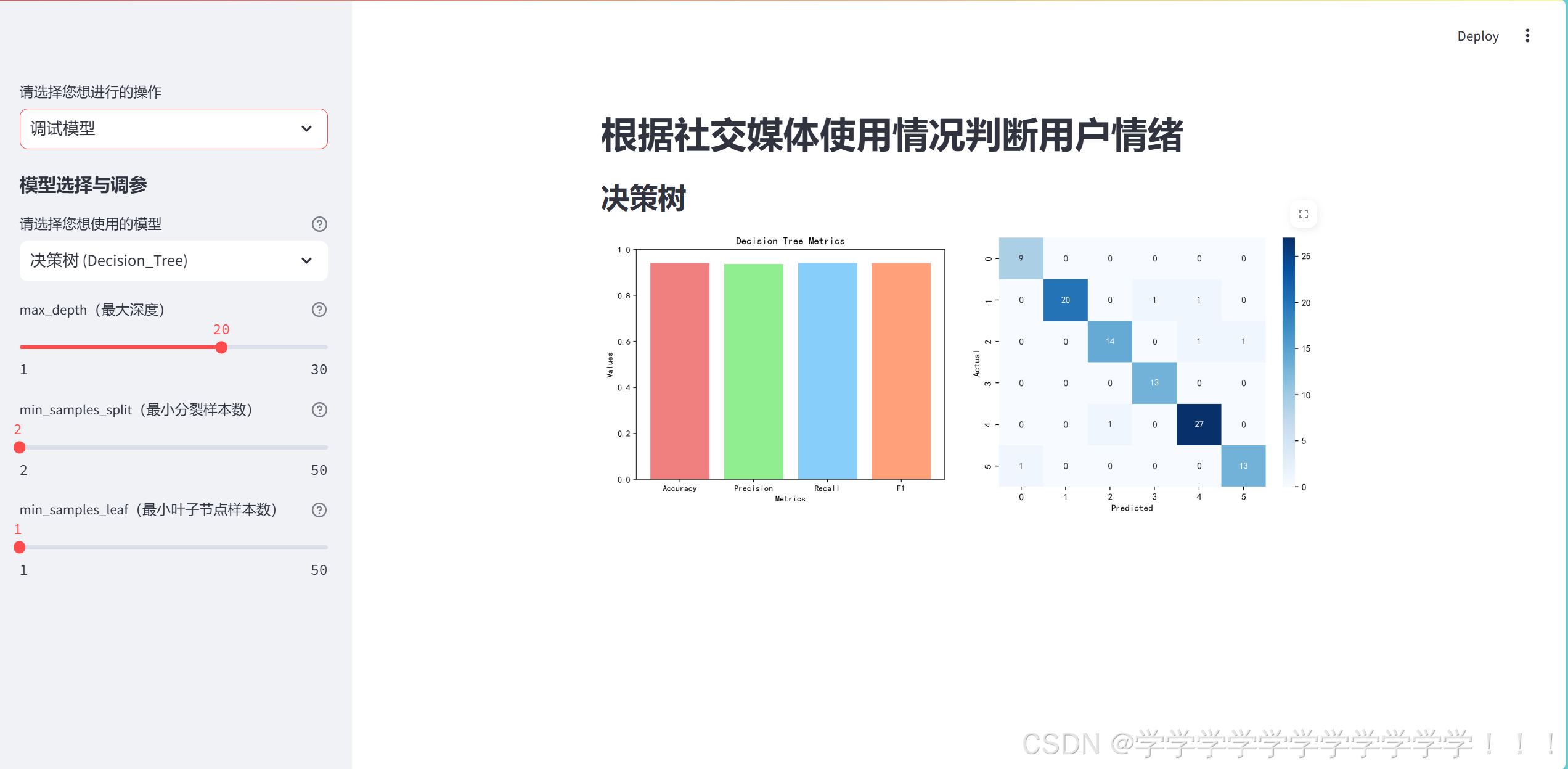
st.pyplot(fig1)这个部分画了两张图,分别代表模型的各种成绩(['Accuracy', 'Precision', 'Recall', 'F1'])和混淆矩阵
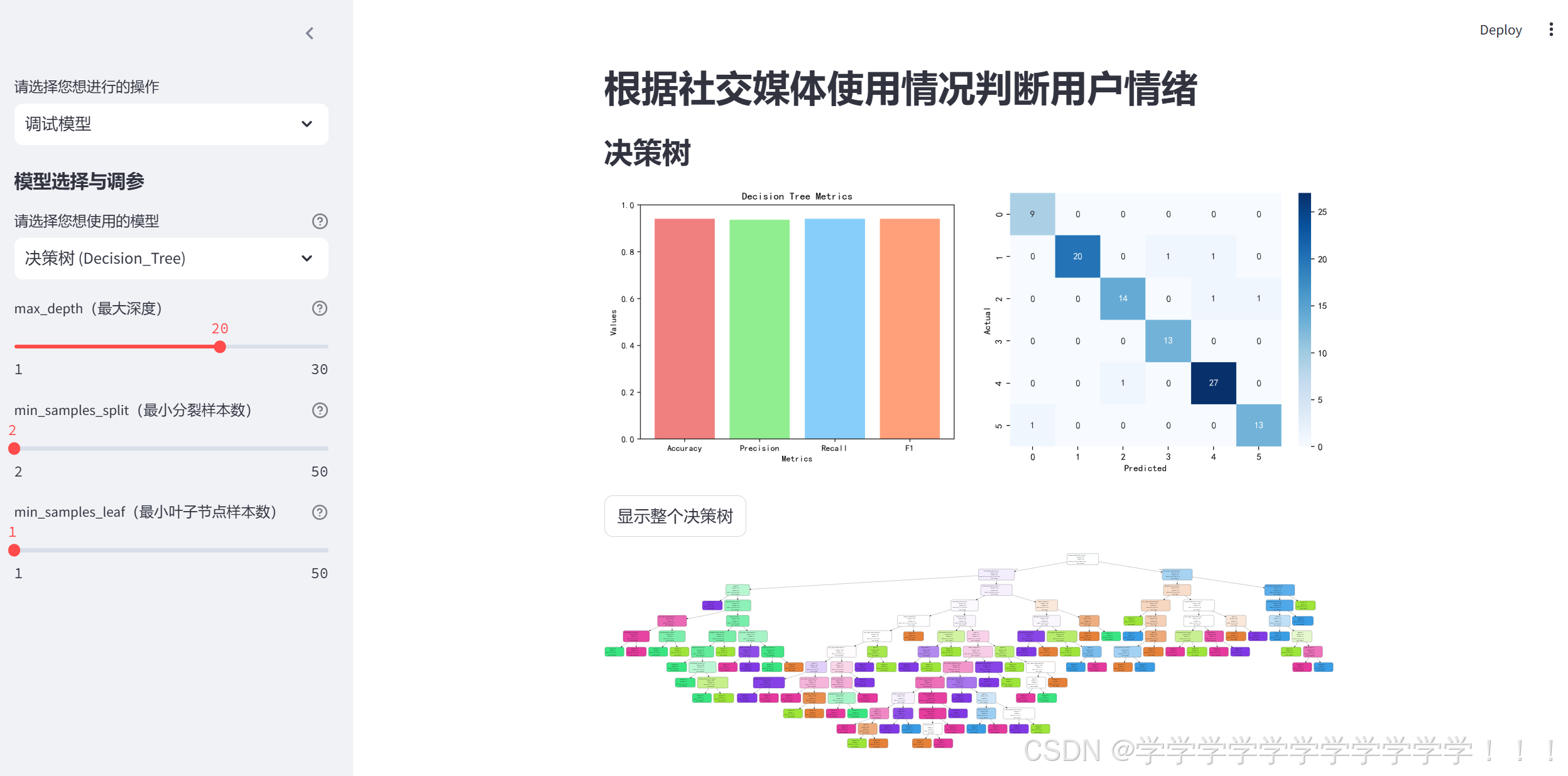
        if st.button('显示整个决策树'):
            with st.spinner('加载中...'):
                time.sleep(0.5)
                target_names = list('Age, Daily_Usage_Time(minutes), Posts_Per_Day, Likes_Received_Per_Day, Comments_Received_Per_Day, Messages_Sent_Per_Day, Gender_Male, Gender_Non - binary, Platform_Instagram, Platform_LinkedIn, Platform_Snapchat, Platform_Telegram, Platform_Twitter, Platform_Whatsapp'.split(","))
                # 将决策树模型导出为graphviz格式的dot文件
                dot_data = export_graphviz(Decision_Tree, out_file=None,
                                           feature_names=target_names,
                                           class_names=list(set(test_y['Dominant_Emotion'])),
                                           filled=True, rounded=True,
                                           special_characters=True)
                # 使用graphviz库的Source函数将dot文件转换为可视化图形
                graph = graphviz.Source(dot_data)
                st.graphviz_chart(dot_data)
这里添加一个显示整个决策树的按钮,点击按钮后会通过export_graphviz()函数画出整个决策树
下面我们可以把写的代码放到页面里,主要是好看,可以充实页面
        st.code('''
            if model == '决策树 (Decision_Tree)':
        st.subheader('决策树')
        iterations = st.sidebar.slider("max_depth(最大深度)", 1, 30, 20, 1, help='决策树的最大深度,限制树的生长,防止过拟合.')
        min_samples_split1 = st.sidebar.slider("min_samples_split(最小分裂样本数)", 2, 50, 2, 1, help='内部节点再划分所需的最小样本数。')
        min_samples_leaf1 = st.sidebar.slider("min_samples_leaf(最小叶子节点样本数)", 1, 50, 1, 1, help='叶节点所需的最小样本数。')

        progress_bar = st.empty()

        with st.spinner('加载中...'):
            time.sleep(0.5)
            # 实例决策树
            Decision_Tree = DecisionTreeClassifier(criterion='entropy', max_depth=iterations, min_samples_split=min_samples_split1, min_samples_leaf=min_samples_leaf1, random_state=2024)
            # 训练决策树
            Decision_Tree.fit(train_x, train_y)
            joblib.dump(Decision_Tree,
                        'D:\social-media-usage-and-emotional-well-being\pythonProject\models\Decision_Tree_model.pickle')
            # 预测
            Decision_Tree_pred = Decision_Tree.predict(test_x)
            # precision成绩
            Decision_Tree_precision = precision_score(test_y, Decision_Tree_pred, average='macro')
            # recall成绩
            Decision_Tree_recall = recall_score(test_y, Decision_Tree_pred, average='micro')
            # f1成绩
            Decision_Tree_f1 = f1_score(test_y, Decision_Tree_pred, average='weighted')
            # 准确率
            Decision_Tree_accuracy = accuracy_score(test_y, Decision_Tree_pred)
            # 混淆矩阵
            conf_matrix = confusion_matrix(test_y, Decision_Tree_pred)
            # 指标名称列表
            metrics = ['Accuracy', 'Precision', 'Recall', 'F1']
            # 对应的指标值列表
            values = [Decision_Tree_accuracy, Decision_Tree_precision, Decision_Tree_recall, Decision_Tree_f1]
            # 绘制条形图
            fig, ax = plt.subplots()
            colors = ['lightcoral', 'lightgreen', 'lightskyblue', 'lightsalmon']
            ax.bar(metrics, values, color=colors)
            # 添加标题
            ax.set_title("Decision Tree Metrics")
            # 添加x轴标签
            ax.set_xlabel("Metrics")
            # 添加y轴标签
            ax.set_ylabel("Values")
            ax.set_ylim(0, 1)
            # 显示图形
            # st.pyplot(fig)

            fig1, ax = plt.subplots()
            sns.heatmap(conf_matrix, annot=True, fmt='d', cmap='Blues')
            ax.set_xlabel('Predicted')
            ax.set_ylabel('Actual')

            # 将两个图放在一行
            col1, col2 = st.columns(2)
            with col1:
                st.pyplot(fig)
            with col2:
                st.pyplot(fig1)

        if st.button('显示整个决策树'):
            with st.spinner('加载中...'):
                time.sleep(0.5)
                target_names = list('Age, Daily_Usage_Time(minutes), Posts_Per_Day, Likes_Received_Per_Day, Comments_Received_Per_Day, Messages_Sent_Per_Day, Gender_Male, Gender_Non - binary, Platform_Instagram, Platform_LinkedIn, Platform_Snapchat, Platform_Telegram, Platform_Twitter, Platform_Whatsapp'.split(","))
                # 将决策树模型导出为graphviz格式的dot文件
                dot_data = export_graphviz(Decision_Tree, out_file=None,
                                           feature_names=target_names,
                                           class_names=list(set(test_y['Dominant_Emotion'])),
                                           filled=True, rounded=True,
                                           special_characters=True)
                # 使用graphviz库的Source函数将dot文件转换为可视化图形
                graph = graphviz.Source(dot_data)
                st.graphviz_chart(dot_data)
        ''')
3.2knn
with st.spinner('加载中...'):
time.sleep(0.5)
knn = KNeighborsClassifier(n_neighbors=n_neighbors, weights=weights2, algorithm=algorithm1, p=p2, leaf_size=leaf_size1)
knn.fit(train_x, train_y)
joblib.dump(knn,
'D:\social-media-usage-and-emotional-well-being\pythonProject\models\knn_model.pickle')
# 预测
knn_pred = knn.predict(test_x)
# 各种成绩
knn_precision = precision_score(test_y, knn_pred, average='macro')
knn_recall = recall_score(test_y, knn_pred, average='micro')
knn_f1 = f1_score(test_y, knn_pred, average='weighted')
knn_accuracy = accuracy_score(test_y, knn_pred)
metrics = ['Accuracy', 'Precision', 'Recall', 'F1']
# 对应的指标值列表
values = [knn_accuracy, knn_precision, knn_recall, knn_f1]
# 绘制条形图
fig, ax = plt.subplots()
colors = ['lightgreen', 'lightsalmon', 'lightskyblue', 'lightcoral', ]
ax.bar(metrics, values, color=colors)
# 添加标题
ax.set_title("Decision Tree Metrics")
# 添加x轴标签
ax.set_xlabel("Metrics")
# 添加y轴标签
ax.set_ylabel("Values")
ax.set_ylim(0, 1)
# 显示图形
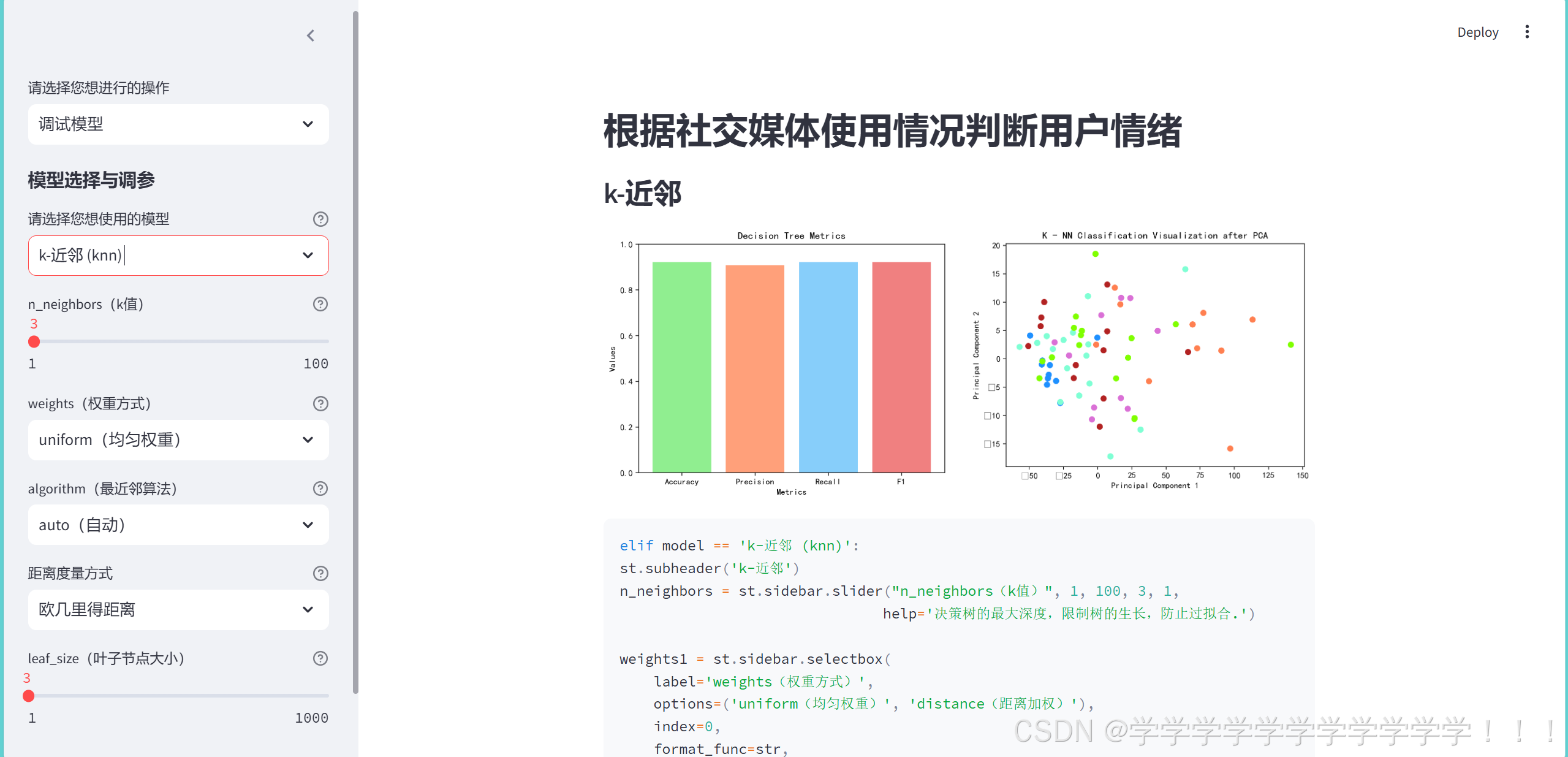
# st.pyplot(fig)同样的,这里训练了knn的模型并且画出了模型各项成绩的图
            pca = PCA(n_components=2)
            newData = pca.fit_transform(test_x)

            # st.write(newData[:, 0])

            colors1 = []
            for i in knn_pred:
                if i == 'Neutral':
                    colors1.append('aquamarine')
                elif i == 'Anxiety':
                    colors1.append('chartreuse')
                elif i == 'Happiness':
                    colors1.append('coral')
                elif i == 'Boredom':
                    colors1.append('dodgerblue')
                elif i == 'Sadness':
                    colors1.append('firebrick')
                elif i == 'Anger':
                    colors1.append('orchid')
            fig3, ax = plt.subplots()
            ax.scatter(newData[:, 0], newData[:, 1], c=colors1, s=40)
            ax.set_title("K - NN Classification Visualization after PCA")
            ax.set_xlabel("Principal Component 1")
            ax.set_ylabel("Principal Component 2")
            # st.pyplot(fig3)
            col1, col2 = st.columns(2)
            with col1:
                st.pyplot(fig)
            with col2:
                st.pyplot(fig3)
这里将测试数据通过pca降维到二维,来画一个knn的直观平面图,这些点的颜色由预测的值决定,然后添加上这部分的代码
        st.code('''
            elif model == 'k-近邻 (knn)':
        st.subheader('k-近邻')
        n_neighbors = st.sidebar.slider("n_neighbors(k值)", 1, 100, 3, 1,
                                       help='决策树的最大深度,限制树的生长,防止过拟合.')

        weights1 = st.sidebar.selectbox(
            label='weights(权重方式)',
            options=('uniform(均匀权重)', 'distance(距离加权)'),
            index=0,
            format_func=str,
            help='用于指定近邻样本的权重计算方式。'
        )
        if weights1 == 'uniform(均匀权重)':
            weights2 = 'uniform'
        else:
            weights2 = 'distance'

        algorithm1 = st.sidebar.selectbox(
            label='algorithm(最近邻算法)',
            options=('auto(自动)', 'ball_tree', 'kd_tree'),
            index=0,
            format_func=str,
            help='用于指定计算最近邻居的算法'
        )
        if algorithm1 == 'auto(自动)':
            algorithm1 = 'auto'

        p1 = st.sidebar.selectbox(
            label='距离度量方式',
            options=('欧几里得距离', '曼哈顿距离'),
            index=0,
            format_func=str,
            help='用于闵可夫斯基距离(metric = "minkowski")的参数。当p = 1时,闵可夫斯基距离就是曼哈顿距离;当p = 2时,就是欧几里得距离。。'
        )
        if p1 == '曼哈顿距离':
            p2 = 1
        else:
            p2 = 2

        leaf_size1 = st.sidebar.slider("leaf_size(叶子节点大小)", 1, 1000, 3, 1, help='这主要是用于 “ball_tree” 和 “kd_tree” 算法中的一个参数,它控制树的叶子节点大小。')
        progress_bar = st.empty()
        with st.spinner('加载中...'):
            time.sleep(0.5)
            knn = KNeighborsClassifier(n_neighbors=n_neighbors, weights=weights2, algorithm=algorithm1, p=p2, leaf_size=leaf_size1)
            knn.fit(train_x, train_y)
            joblib.dump(knn,
                        'D:\social-media-usage-and-emotional-well-being\pythonProject\models\knn_model.pickle')
            # 预测
            knn_pred = knn.predict(test_x)
            # 各种成绩
            knn_precision = precision_score(test_y, knn_pred, average='macro')
            knn_recall = recall_score(test_y, knn_pred, average='micro')
            knn_f1 = f1_score(test_y, knn_pred, average='weighted')
            knn_accuracy = accuracy_score(test_y, knn_pred)

            metrics = ['Accuracy', 'Precision', 'Recall', 'F1']
            # 对应的指标值列表
            values = [knn_accuracy, knn_precision, knn_recall, knn_f1]
            # 绘制条形图
            fig, ax = plt.subplots()
            colors = ['lightgreen', 'lightsalmon', 'lightskyblue', 'lightcoral', ]
            ax.bar(metrics, values, color=colors)
            # 添加标题
            ax.set_title("Decision Tree Metrics")
            # 添加x轴标签
            ax.set_xlabel("Metrics")
            # 添加y轴标签
            ax.set_ylabel("Values")
            ax.set_ylim(0, 1)
            # 显示图形
            # st.pyplot(fig)

            pca = PCA(n_components=2)
            newData = pca.fit_transform(test_x)

            # st.write(newData[:, 0])

            colors1 = []
            for i in knn_pred:
                if i == 'Neutral':
                    colors1.append('aquamarine')
                elif i == 'Anxiety':
                    colors1.append('chartreuse')
                elif i == 'Happiness':
                    colors1.append('coral')
                elif i == 'Boredom':
                    colors1.append('dodgerblue')
                elif i == 'Sadness':
                    colors1.append('firebrick')
                elif i == 'Anger':
                    colors1.append('orchid')
            fig3, ax = plt.subplots()
            ax.scatter(newData[:, 0], newData[:, 1], c=colors1, s=40)
            ax.set_title("K - NN Classification Visualization after PCA")
            ax.set_xlabel("Principal Component 1")
            ax.set_ylabel("Principal Component 2")
            # st.pyplot(fig3)
            col1, col2 = st.columns(2)
            with col1:
                st.pyplot(fig)
            with col2:
                st.pyplot(fig3)
        ''')
最后的效果是这样的
3.3支持向量机
        svm = SVC(C=c, kernel=kernel, gamma='scale', shrinking=shrinking, probability=probability)
        svm.fit(train_x, train_y)
        joblib.dump(svm,
                    'D:\social-media-usage-and-emotional-well-being\pythonProject\models\svm_model.pickle')
        svm_pred = svm.predict(test_x)
        svm_precision = precision_score(test_y, svm_pred, average='macro')
        svm_recall = recall_score(test_y, svm_pred, average='micro')
        svm_f1 = f1_score(test_y, svm_pred, average='weighted')
        svm_accuracy = accuracy_score(test_y, svm_pred)

        metrics = ['Accuracy', 'Precision', 'Recall', 'F1']
        # 对应的指标值列表
        values = [svm_accuracy, svm_precision, svm_recall, svm_f1]
        # 绘制条形图
        fig, ax = plt.subplots()
        colors = ['lightgreen', 'lightsalmon', 'lightskyblue', 'lightcoral', ]
        ax.bar(metrics, values, color=colors)
        # 添加标题
        ax.set_title("Decision Tree Metrics")
        # 添加x轴标签
        ax.set_xlabel("Metrics")
        # 添加y轴标签
        ax.set_ylabel("Values")
        ax.set_ylim(0, 1)
        # 显示图形
        st.pyplot(fig)
还是一样,先画了模型的各种成绩的直方图,方便调试模型,接下来画支持向量机的3D散点图,还有要特别注意的是,支持向量机的核选为'linear(线性核)', 'polynomial(多项式核)'的时候,运行会非常慢,因为这两个核都需要大量的计算成本,特别是选择线性核,还把惩罚参数C设定的特别大的时候等的时间就特别特别长,这边建议谨慎
        if st.button('显示3D散点模型'):
            with st.spinner('加载中...'):
                # 创建PCA对象,指定降维到3个主成分

                pca = PCA(n_components=3)

                # 对训练集和测试集都执行降维操作
                train_x_pca = pca.fit_transform(train_x)
                test_x_pca = pca.transform(test_x)

                # 创建三维坐标轴对象
                fig1 = plt.figure(figsize=(10, 8))
                # 修改此处,确保使用正确的图形对象来添加坐标轴
                ax = fig1.add_subplot(111, projection='3d')

                # 获取不同类别对应的索引
                unique_classes = np.unique(train_y)
                colors = ['r', 'g', 'b']  # 为不同类别设置不同颜色

                # 绘制训练集数据点
                for class_idx, color in zip(unique_classes, colors):
                    class_mask = train_y == class_idx
                    # 这里修改索引方式,通过循环每个样本进行正确索引
                    for sample_idx in np.where(class_mask)[0]:
                        ax.scatter(train_x_pca[sample_idx, 0], train_x_pca[sample_idx, 1], train_x_pca[sample_idx, 2],
                                   c=color)

                # 绘制测试集数据点(可选择以不同样式展示,比如用空心圆等,便于区分训练集和测试集)
                for class_idx, color in zip(unique_classes, colors):
                    class_mask = test_y == class_idx
                    for sample_idx in np.where(class_mask)[0]:
                        ax.scatter(test_x_pca[sample_idx, 0], test_x_pca[sample_idx, 1], test_x_pca[sample_idx, 2],
                                   c=color, marker='o', facecolors='none', edgecolors=color )

                # 设置坐标轴标签
                ax.set_xlabel('Principal Component 1')
                ax.set_ylabel('Principal Component 2')
                ax.set_zlabel('Principal Component 3')
                ax.set_title('SVM Classification Visualization in 3D (After PCA)')
                ax.legend()

                # 在Streamlit中展示图形
                st.pyplot(fig1)
这部分可能比较难,我自己写的时候调试了不少时间,这里建议还是添加一个按钮,按了之后才显示散点图,因为画这个图也需要不少时间,有点慢,最好再前面加一个“加载中”,防止用户为有bug
        st.code('''
            elif model == '支持向量机 (SVM)':
        st.subheader('支持向量机')

        kernel = st.sidebar.selectbox(
            label='kernel(核函数类型)',
            options=('rbf(径向基函数核)', 'linear(线性核)', 'polynomial(多项式核)'),
            index=0,
            format_func=str,
            help='核函数类型'
        )
        if kernel == 'rbf(径向基函数核)':
            kernel = 'rbf'
            c = st.sidebar.slider("C(惩罚参数)", 1, 10000, 10000, 1,
                                  help='控制对错误分类的惩罚程度')

        elif kernel == 'linear(线性核)':
            kernel = 'linear'
            c = st.sidebar.slider("C(惩罚参数)", 1, 10, 1, 1,
                                  help='控制对错误分类的惩罚程度')

        else:
            kernel = 'poly'
            c = st.sidebar.slider("C(惩罚参数)", 1, 1000, 100, 1,
                                  help='控制对错误分类的惩罚程度')

        shrinking = st.sidebar.selectbox(
            label='shrinking(是否使用收缩启发式)',
            options=(True, False),
            index=0,
            format_func=str,
            help='在训练过程中可能会改变优化算法的行为,不使用收缩启发式可能会使训练时间变长,但在某些特定情况下可能会提高模型的稳定性或者准确性。'
        )

        probability = st.sidebar.selectbox(
            label='probability(是否启用概率估计)',
            options=(True, False),
            index=0,
            format_func=str,
            help='在训练过程中可能会改变优化算法的行为,不使用收缩启发式可能会使训练时间变长,但在某些特定情况下可能会提高模型的稳定性或者准确性。'
        )

        svm = SVC(C=c, kernel=kernel, gamma='scale', shrinking=shrinking, probability=probability)
        svm.fit(train_x, train_y)
        joblib.dump(svm,
                    'D:\social-media-usage-and-emotional-well-being\pythonProject\models\svm_model.pickle')
        svm_pred = svm.predict(test_x)
        svm_precision = precision_score(test_y, svm_pred, average='macro')
        svm_recall = recall_score(test_y, svm_pred, average='micro')
        svm_f1 = f1_score(test_y, svm_pred, average='weighted')
        svm_accuracy = accuracy_score(test_y, svm_pred)

        metrics = ['Accuracy', 'Precision', 'Recall', 'F1']
        # 对应的指标值列表
        values = [svm_accuracy, svm_precision, svm_recall, svm_f1]
        # 绘制条形图
        fig, ax = plt.subplots()
        colors = ['lightgreen', 'lightsalmon', 'lightskyblue', 'lightcoral', ]
        ax.bar(metrics, values, color=colors)
        # 添加标题
        ax.set_title("Decision Tree Metrics")
        # 添加x轴标签
        ax.set_xlabel("Metrics")
        # 添加y轴标签
        ax.set_ylabel("Values")
        ax.set_ylim(0, 1)
        # 显示图形
        st.pyplot(fig)
        if st.button('显示3D散点模型'):
            with st.spinner('加载中...'):
                # 创建PCA对象,指定降维到3个主成分

                pca = PCA(n_components=3)

                # 对训练集和测试集都执行降维操作
                train_x_pca = pca.fit_transform(train_x)
                test_x_pca = pca.transform(test_x)

                # 创建三维坐标轴对象
                fig1 = plt.figure(figsize=(10, 8))
                # 修改此处,确保使用正确的图形对象来添加坐标轴
                ax = fig1.add_subplot(111, projection='3d')

                # 获取不同类别对应的索引
                unique_classes = np.unique(train_y)
                colors = ['r', 'g', 'b']  # 为不同类别设置不同颜色

                # 绘制训练集数据点
                for class_idx, color in zip(unique_classes, colors):
                    class_mask = train_y == class_idx
                    # 这里修改索引方式,通过循环每个样本进行正确索引
                    for sample_idx in np.where(class_mask)[0]:
                        ax.scatter(train_x_pca[sample_idx, 0], train_x_pca[sample_idx, 1], train_x_pca[sample_idx, 2],
                                   c=color)

                # 绘制测试集数据点(可选择以不同样式展示,比如用空心圆等,便于区分训练集和测试集)
                for class_idx, color in zip(unique_classes, colors):
                    class_mask = test_y == class_idx
                    for sample_idx in np.where(class_mask)[0]:
                        ax.scatter(test_x_pca[sample_idx, 0], test_x_pca[sample_idx, 1], test_x_pca[sample_idx, 2],
                                   c=color, marker='o', facecolors='none', edgecolors=color )

                # 设置坐标轴标签
                ax.set_xlabel('Principal Component 1')
                ax.set_ylabel('Principal Component 2')
                ax.set_zlabel('Principal Component 3')
                ax.set_title('SVM Classification Visualization in 3D (After PCA)')
                ax.legend()

                # 在Streamlit中展示图形
                st.pyplot(fig1)
        ''')
添加上这部分的代码
3.4集成学习
3.4.1基础学习器
    elif model == '集成学习 (Ensemble Learning)':

        st.subheader("集成学习")
        st.sidebar.subheader('基础学习器')
        base_model = st.sidebar.selectbox(
            label='选择基础学习器',
            options=('Decision_Tree', 'knn'),
            index=0,
            format_func=str,
            help='在训练过程中可能会改变优化算法的行为,不使用收缩启发式可能会使训练时间变长,但在某些特定情况下可能会提高模型的稳定性或者准确性。'
        )


        #决策树
        if base_model=="Decision_Tree":
            iterations = st.sidebar.slider("max_depth(最大深度)", 1, 30, 20, 1,
                                           help='决策树的最大深度,限制树的生长,防止过拟合.')
            min_samples_split1 = st.sidebar.slider("min_samples_split(最小分裂样本数)", 2, 50, 2, 1,
                                                   help='内部节点再划分所需的最小样本数。')
            min_samples_leaf1 = st.sidebar.slider("min_samples_leaf(最小叶子节点样本数)", 1, 50, 1, 1,
                                                  help='叶节点所需的最小样本数。')
            base_clf = DecisionTreeClassifier(criterion='entropy', max_depth=iterations,
                                              min_samples_split=min_samples_split1, min_samples_leaf=min_samples_leaf1,
                                              random_state=2024)
            base_clf.fit(train_x, train_y)
            joblib.dump(base_clf,
                        r'D:\social-media-usage-and-emotional-well-being\pythonProject\models\base_clf.pickle')


        else:
            n_neighbors = st.sidebar.slider("n_neighbors(k值)", 1, 100, 3, 1,
                                            help='决策树的最大深度,限制树的生长,防止过拟合.')

            weights1 = st.sidebar.selectbox(
                label='weights(权重方式)',
                options=('uniform(均匀权重)', 'distance(距离加权)'),
                index=0,
                format_func=str,
                help='用于指定近邻样本的权重计算方式。'
            )
            if weights1 == 'uniform(均匀权重)':
                weights2 = 'uniform'
            else:
                weights2 = 'distance'

            algorithm1 = st.sidebar.selectbox(
                label='algorithm(最近邻算法)',
                options=('auto(自动)', 'ball_tree', 'kd_tree'),
                index=0,
                format_func=str,
                help='用于指定计算最近邻居的算法'
            )
            if algorithm1 == 'auto(自动)':
                algorithm1 = 'auto'

            p1 = st.sidebar.selectbox(
                label='距离度量方式',
                options=('欧几里得距离', '曼哈顿距离'),
                index=0,
                format_func=str,
                help='用于闵可夫斯基距离(metric = "minkowski")的参数。当p = 1时,闵可夫斯基距离就是曼哈顿距离;当p = 2时,就是欧几里得距离。。'
            )
            if p1 == '曼哈顿距离':
                p2 = 1
            else:
                p2 = 2

            leaf_size1 = st.sidebar.slider("leaf_size(叶子节点大小)", 1, 1000, 3, 1,
                                           help='这主要是用于 “ball_tree” 和 “kd_tree” 算法中的一个参数,它控制树的叶子节点大小。')
            base_clf = KNeighborsClassifier(n_neighbors=n_neighbors, weights=weights2, algorithm=algorithm1, p=p2, leaf_size=leaf_size1)
            base_clf.fit(train_x, train_y)
            joblib.dump(base_clf,
                        r'D:\social-media-usage-and-emotional-well-being\pythonProject\models\base_clf.pickle')

            pca = PCA(n_components=2)
            newData = pca.fit_transform(test_x)
这个部分是对基础学习器的设置,这里设置了两个基础学习器(决策树和knn)没有选支持向量机是因为训练成本太大,耗时太长
3.4.2 集成学习器
st.sidebar.subheader('集成分类器')
n_estimators = st.sidebar.slider("n_estimators(基学习器的数量)", 1, 30, 10, 1,
help='这个参数是可以调整的重要参数。它决定了集成学习中基学习器(例如决策树)的数量。增加n_estimators通常可以提高模型的性能和稳定性,但也会增加计算成本和训练时间。例如,当处理一个复杂的分类问题,数据有较多的噪声和特征时,适当增加n_estimators可能会使模型更好地拟合数据。')
max_samples = st.sidebar.slider("max_samples(抽样的样本比例)", 0.0, 1.0, 1.0, format="%.2f",
help='用于控制每次构建基学习器时从训练数据集中抽样的样本比例(如果值小于 1.0)或样本数量(如果值为整数)。调整这个参数可以改变基学习器训练数据的多样性。如果数据量很大,适当减小max_samples可以减少每个基学习器的训练时间,同时增加基学习器之间的差异。')
max_features = st.sidebar.slider("max_samples(抽样的样本比例)", 0.0, 1.0, 1.0, format="%.2f",
help='控制每次构建基学习器时从特征集合中抽取的特征比例(如果值小于 1.0)或特征数量(如果值为整数)。通过调整这个参数可以引入特征的随机性,特别是在特征维度较高的情况下,能够防止模型过度依赖某些特征,提高模型的泛化能力。')
bootstrap = st.sidebar.selectbox(
label='bootstrap(是否采用有放回基学习器)',
options=(True, False),
index=0,
format_func=str,
help='在训练过程中可能会改变优化算法的行为,不使用收缩启发式可能会使训练时间变长,但在某些特定情况下可能会提高模型的稳定性或者准确性。'
)
bootstrap_features = st.sidebar.selectbox(
label='bootstrap(是否采用有放回特征)',
options=(True, False),
index=0,
format_func=str,
help='在训练过程中可能会改变优化算法的行为,不使用收缩启发式可能会使训练时间变长,但在某些特定情况下可能会提高模型的稳定性或者准确性。'
)
with st.spinner('加载中...'):
time.sleep(0.5)
bagging_clf = BaggingClassifier(base_clf, n_estimators=n_estimators, max_samples=max_samples, max_features=max_features, bootstrap=bootstrap, bootstrap_features=bootstrap_features, random_state=42)
bagging_clf.fit(train_x, train_y)
joblib.dump(bagging_clf,
r'D:\social-media-usage-and-emotional-well-being\pythonProject\models\bagging_clf.pickle')
# 训练基础分类器模型
y_pred_base_clf = base_clf.predict(test_x)
y_pred_bagging = bagging_clf.predict(test_x)
bagging_clf_precision = precision_score(test_y, y_pred_bagging, average='macro')
bagging_clf_recall = recall_score(test_y, y_pred_bagging, average='micro')
bagging_clf_f1 = f1_score(test_y, y_pred_bagging, average='weighted')
bagging_clf_accuracy = accuracy_score(test_y, y_pred_bagging)
metrics = ['Accuracy', 'Precision', 'Recall', 'F1']
# 对应的指标值列表
values = [bagging_clf_accuracy, bagging_clf_precision, bagging_clf_recall, bagging_clf_f1]
# 绘制条形图
fig, ax = plt.subplots()
colors = ['lightgreen', 'lightsalmon', 'lightskyblue', 'lightcoral' ]
ax.bar(metrics, values, color=colors)
# 添加标题
ax.set_title("集成学习器")
# 添加x轴标签
ax.set_xlabel("Metrics")
# 添加y轴标签
ax.set_ylabel("Values")
ax.set_ylim(0, 1)
# 显示图形
# st.pyplot(fig)
base_clf_precision = precision_score(test_y, y_pred_base_clf, average='macro')
base_clf_recall = recall_score(test_y, y_pred_base_clf, average='micro')
base_clf_f1 = f1_score(test_y, y_pred_base_clf, average='weighted')
base_clf_accuracy = accuracy_score(test_y, y_pred_base_clf)
metrics = ['Accuracy', 'Precision', 'Recall', 'F1']
# 对应的指标值列表
values = [base_clf_accuracy, base_clf_precision, base_clf_recall, base_clf_f1]
# 绘制条形图
fig1, ax = plt.subplots()
colors = ['lightgreen', 'lightsalmon', 'lightskyblue', 'lightcoral']
ax.bar(metrics, values, color=colors)
# 添加标题
ax.set_title("基础学习器")
# 添加x轴标签
ax.set_xlabel("Metrics")
# 添加y轴标签
ax.set_ylabel("Values")
ax.set_ylim(0, 1)
# 显示图形
# st.pyplot(fig)
col1, col2 = st.columns(2)
with col1:
st.pyplot(fig)
with col2:
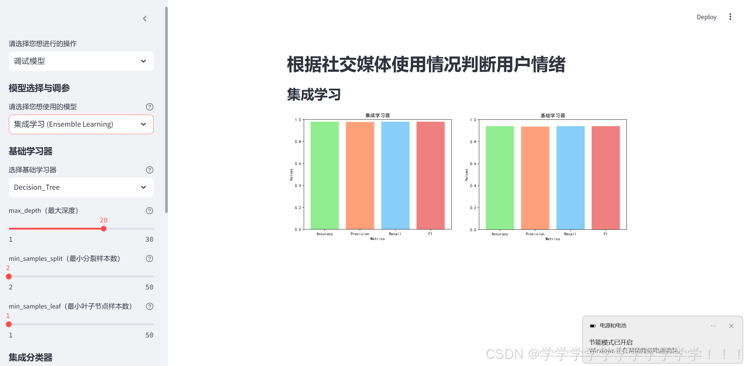
st.pyplot(fig1)这里先对基础学习器进行训练,再对集成分类器进行训练,并把基础学习器和集成学习器的准确度等模型成绩加上,方便调参
下面是图示部分,可以把基础学习器的训练效果图写上去
            if base_model == "Decision_Tree":

                cb = st.checkbox('显示决策树', value=False)

                if cb:
                    with st.spinner('加载中...'):
                        time.sleep(0.5)
                        target_names = list(
                            'Age, Daily_Usage_Time(minutes), Posts_Per_Day, Likes_Received_Per_Day, Comments_Received_Per_Day, Messages_Sent_Per_Day, Gender_Male, Gender_Non - binary, Platform_Instagram, Platform_LinkedIn, Platform_Snapchat, Platform_Telegram, Platform_Twitter, Platform_Whatsapp'.split(
                                ","))
                        # 将决策树模型导出为graphviz格式的dot文件
                        dot_data = export_graphviz(base_clf, out_file=None,
                                                   feature_names=target_names,
                                                   class_names=list(set(test_y['Dominant_Emotion'])),
                                                   filled=True, rounded=True,
                                                   special_characters=True)
                        # 使用graphviz库的Source函数将dot文件转换为可视化图形
                        graph = graphviz.Source(dot_data)
                        st.graphviz_chart(dot_data)

            else:
                # st.write(newData[:, 0])
                cb1 = st.checkbox('显示knn', value=False)

                if cb1:
                    colors1 = []
                    for i in y_pred_base_clf:
                        if i == 'Neutral':
                            colors1.append('aquamarine')
                        elif i == 'Anxiety':
                            colors1.append('chartreuse')
                        elif i == 'Happiness':
                            colors1.append('coral')
                        elif i == 'Boredom':
                            colors1.append('dodgerblue')
                        elif i == 'Sadness':
                            colors1.append('firebrick')
                        elif i == 'Anger':
                            colors1.append('orchid')
                    pca = PCA(n_components=2)
                    newData = pca.fit_transform(test_x)
                    fig3, ax = plt.subplots()
                    ax.scatter(newData[:, 0], newData[:, 1], c=colors1, s=40)
                    ax.set_title("K - NN Classification Visualization after PCA")
                    ax.set_xlabel("Principal Component 1")
                    ax.set_ylabel("Principal Component 2")
                    st.pyplot(fig3)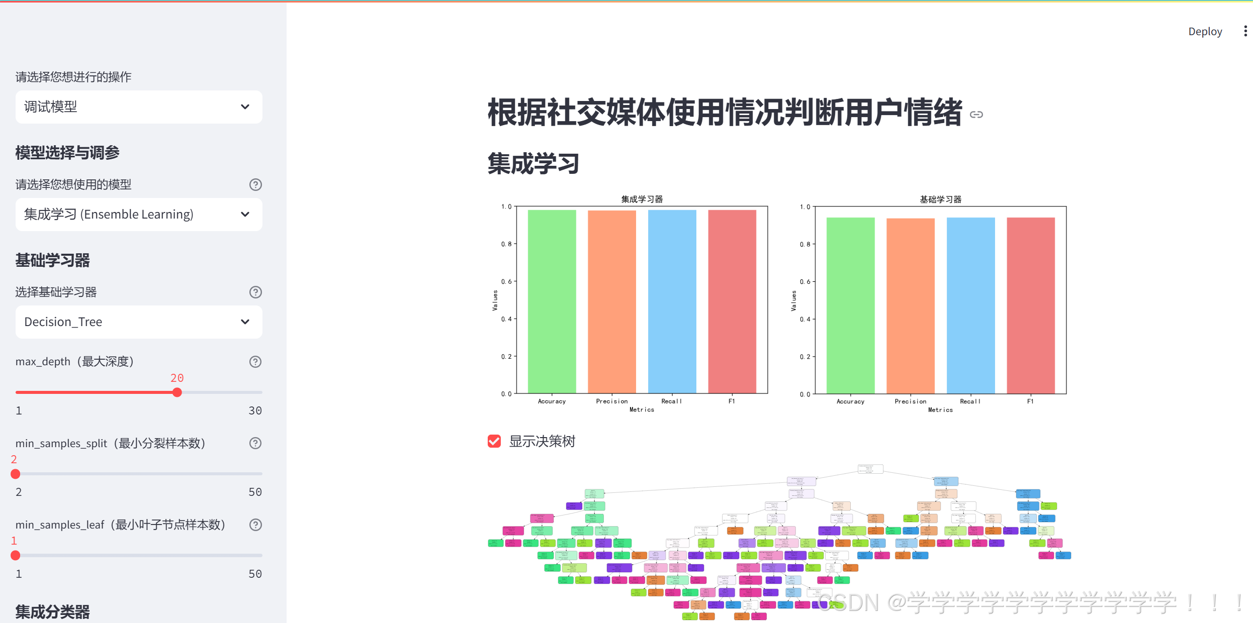

当然别忘了放置代码
            st.code('''
                elif model == '集成学习 (Ensemble Learning)':

        st.subheader("集成学习")
        st.sidebar.subheader('基础学习器')
        base_model = st.sidebar.selectbox(
            label='选择基础学习器',
            options=('Decision_Tree', 'knn'),
            index=0,
            format_func=str,
            help='在训练过程中可能会改变优化算法的行为,不使用收缩启发式可能会使训练时间变长,但在某些特定情况下可能会提高模型的稳定性或者准确性。'
        )


        #决策树
        if base_model=="Decision_Tree":
            iterations = st.sidebar.slider("max_depth(最大深度)", 1, 30, 20, 1,
                                           help='决策树的最大深度,限制树的生长,防止过拟合.')
            min_samples_split1 = st.sidebar.slider("min_samples_split(最小分裂样本数)", 2, 50, 2, 1,
                                                   help='内部节点再划分所需的最小样本数。')
            min_samples_leaf1 = st.sidebar.slider("min_samples_leaf(最小叶子节点样本数)", 1, 50, 1, 1,
                                                  help='叶节点所需的最小样本数。')
            base_clf = DecisionTreeClassifier(criterion='entropy', max_depth=iterations,
                                              min_samples_split=min_samples_split1, min_samples_leaf=min_samples_leaf1,
                                              random_state=2024)
            base_clf.fit(train_x, train_y)
            joblib.dump(base_clf,
                        r'D:\social-media-usage-and-emotional-well-being\pythonProject\models\base_clf.pickle')


        else:
            n_neighbors = st.sidebar.slider("n_neighbors(k值)", 1, 100, 3, 1,
                                            help='决策树的最大深度,限制树的生长,防止过拟合.')

            weights1 = st.sidebar.selectbox(
                label='weights(权重方式)',
                options=('uniform(均匀权重)', 'distance(距离加权)'),
                index=0,
                format_func=str,
                help='用于指定近邻样本的权重计算方式。'
            )
            if weights1 == 'uniform(均匀权重)':
                weights2 = 'uniform'
            else:
                weights2 = 'distance'

            algorithm1 = st.sidebar.selectbox(
                label='algorithm(最近邻算法)',
                options=('auto(自动)', 'ball_tree', 'kd_tree'),
                index=0,
                format_func=str,
                help='用于指定计算最近邻居的算法'
            )
            if algorithm1 == 'auto(自动)':
                algorithm1 = 'auto'

            p1 = st.sidebar.selectbox(
                label='距离度量方式',
                options=('欧几里得距离', '曼哈顿距离'),
                index=0,
                format_func=str,
                help='用于闵可夫斯基距离(metric = "minkowski")的参数。当p = 1时,闵可夫斯基距离就是曼哈顿距离;当p = 2时,就是欧几里得距离。。'
            )
            if p1 == '曼哈顿距离':
                p2 = 1
            else:
                p2 = 2

            leaf_size1 = st.sidebar.slider("leaf_size(叶子节点大小)", 1, 1000, 3, 1,
                                           help='这主要是用于 “ball_tree” 和 “kd_tree” 算法中的一个参数,它控制树的叶子节点大小。')
            base_clf = KNeighborsClassifier(n_neighbors=n_neighbors, weights=weights2, algorithm=algorithm1, p=p2, leaf_size=leaf_size1)
            base_clf.fit(train_x, train_y)
            joblib.dump(base_clf,
                        r'D:\social-media-usage-and-emotional-well-being\pythonProject\models\base_clf.pickle')

            pca = PCA(n_components=2)
            newData = pca.fit_transform(test_x)


        st.sidebar.subheader('集成分类器')
        n_estimators = st.sidebar.slider("n_estimators(基学习器的数量)", 1, 30, 10, 1,
                                       help='这个参数是可以调整的重要参数。它决定了集成学习中基学习器(例如决策树)的数量。增加n_estimators通常可以提高模型的性能和稳定性,但也会增加计算成本和训练时间。例如,当处理一个复杂的分类问题,数据有较多的噪声和特征时,适当增加n_estimators可能会使模型更好地拟合数据。')
        max_samples = st.sidebar.slider("max_samples(抽样的样本比例)", 0.0, 1.0, 1.0, format="%.2f",
                                       help='用于控制每次构建基学习器时从训练数据集中抽样的样本比例(如果值小于 1.0)或样本数量(如果值为整数)。调整这个参数可以改变基学习器训练数据的多样性。如果数据量很大,适当减小max_samples可以减少每个基学习器的训练时间,同时增加基学习器之间的差异。')
        max_features = st.sidebar.slider("max_samples(抽样的样本比例)", 0.0, 1.0, 1.0, format="%.2f",
                                       help='控制每次构建基学习器时从特征集合中抽取的特征比例(如果值小于 1.0)或特征数量(如果值为整数)。通过调整这个参数可以引入特征的随机性,特别是在特征维度较高的情况下,能够防止模型过度依赖某些特征,提高模型的泛化能力。')
        bootstrap = st.sidebar.selectbox(
            label='bootstrap(是否采用有放回基学习器)',
            options=(True, False),
            index=0,
            format_func=str,
            help='在训练过程中可能会改变优化算法的行为,不使用收缩启发式可能会使训练时间变长,但在某些特定情况下可能会提高模型的稳定性或者准确性。'
        )
        bootstrap_features = st.sidebar.selectbox(
            label='bootstrap(是否采用有放回特征)',
            options=(True, False),
            index=0,
            format_func=str,
            help='在训练过程中可能会改变优化算法的行为,不使用收缩启发式可能会使训练时间变长,但在某些特定情况下可能会提高模型的稳定性或者准确性。'
        )


        with st.spinner('加载中...'):
            time.sleep(0.5)

            bagging_clf = BaggingClassifier(base_clf, n_estimators=n_estimators, max_samples=max_samples, max_features=max_features, bootstrap=bootstrap, bootstrap_features=bootstrap_features, random_state=42)
            bagging_clf.fit(train_x, train_y)
            joblib.dump(bagging_clf,
                        r'D:\social-media-usage-and-emotional-well-being\pythonProject\models\bagging_clf.pickle')

            # 训练基础分类器模型


            y_pred_base_clf = base_clf.predict(test_x)
            y_pred_bagging = bagging_clf.predict(test_x)

            bagging_clf_precision = precision_score(test_y, y_pred_bagging, average='macro')
            bagging_clf_recall = recall_score(test_y, y_pred_bagging, average='micro')
            bagging_clf_f1 = f1_score(test_y, y_pred_bagging, average='weighted')
            bagging_clf_accuracy = accuracy_score(test_y, y_pred_bagging)

            metrics = ['Accuracy', 'Precision', 'Recall', 'F1']
            # 对应的指标值列表
            values = [bagging_clf_accuracy, bagging_clf_precision, bagging_clf_recall, bagging_clf_f1]
            # 绘制条形图
            fig, ax = plt.subplots()
            colors = ['lightgreen', 'lightsalmon', 'lightskyblue', 'lightcoral' ]
            ax.bar(metrics, values, color=colors)
            # 添加标题
            ax.set_title("集成学习器")
            # 添加x轴标签
            ax.set_xlabel("Metrics")
            # 添加y轴标签
            ax.set_ylabel("Values")
            ax.set_ylim(0, 1)
            # 显示图形
            # st.pyplot(fig)

            base_clf_precision = precision_score(test_y, y_pred_base_clf, average='macro')
            base_clf_recall = recall_score(test_y, y_pred_base_clf, average='micro')
            base_clf_f1 = f1_score(test_y, y_pred_base_clf, average='weighted')
            base_clf_accuracy = accuracy_score(test_y, y_pred_base_clf)

            metrics = ['Accuracy', 'Precision', 'Recall', 'F1']
            # 对应的指标值列表
            values = [base_clf_accuracy, base_clf_precision, base_clf_recall, base_clf_f1]
            # 绘制条形图
            fig1, ax = plt.subplots()
            colors = ['lightgreen', 'lightsalmon', 'lightskyblue', 'lightcoral']
            ax.bar(metrics, values, color=colors)
            # 添加标题
            ax.set_title("基础学习器")
            # 添加x轴标签
            ax.set_xlabel("Metrics")
            # 添加y轴标签
            ax.set_ylabel("Values")
            ax.set_ylim(0, 1)
            # 显示图形
            # st.pyplot(fig)
            col1, col2 = st.columns(2)
            with col1:
                st.pyplot(fig)
            with col2:
                st.pyplot(fig1)

            if base_model == "Decision_Tree":

                cb = st.checkbox('显示决策树', value=False)

                if cb:
                    with st.spinner('加载中...'):
                        time.sleep(0.5)
                        target_names = list(
                            'Age, Daily_Usage_Time(minutes), Posts_Per_Day, Likes_Received_Per_Day, Comments_Received_Per_Day, Messages_Sent_Per_Day, Gender_Male, Gender_Non - binary, Platform_Instagram, Platform_LinkedIn, Platform_Snapchat, Platform_Telegram, Platform_Twitter, Platform_Whatsapp'.split(
                                ","))
                        # 将决策树模型导出为graphviz格式的dot文件
                        dot_data = export_graphviz(base_clf, out_file=None,
                                                   feature_names=target_names,
                                                   class_names=list(set(test_y['Dominant_Emotion'])),
                                                   filled=True, rounded=True,
                                                   special_characters=True)
                        # 使用graphviz库的Source函数将dot文件转换为可视化图形
                        graph = graphviz.Source(dot_data)
                        st.graphviz_chart(dot_data)

            else:
                # st.write(newData[:, 0])
                cb1 = st.checkbox('显示knn', value=False)

                if cb1:
                    colors1 = []
                    for i in y_pred_base_clf:
                        if i == 'Neutral':
                            colors1.append('aquamarine')
                        elif i == 'Anxiety':
                            colors1.append('chartreuse')
                        elif i == 'Happiness':
                            colors1.append('coral')
                        elif i == 'Boredom':
                            colors1.append('dodgerblue')
                        elif i == 'Sadness':
                            colors1.append('firebrick')
                        elif i == 'Anger':
                            colors1.append('orchid')
                    pca = PCA(n_components=2)
                    newData = pca.fit_transform(test_x)
                    fig3, ax = plt.subplots()
                    ax.scatter(newData[:, 0], newData[:, 1], c=colors1, s=40)
                    ax.set_title("K - NN Classification Visualization after PCA")
                    ax.set_xlabel("Principal Component 1")
                    ax.set_ylabel("Principal Component 2")
                    st.pyplot(fig3)
            ''',language='python')
4.情绪预测部分
else:
    # st.sidebar.subheader('集成分类器')
    pred_model = st.sidebar.selectbox(
        label='请输入您想使用的预测魔性',
        options=('决策树 (Decision_Tree)', 'k-近邻 (knn)', '支持向量机 (SVM)', '集成学习 (Ensemble Learning)'),
        index=0,
        format_func=str,
        help='目前只提供这四种模型'
    )
    if pred_model == '决策树 (Decision_Tree)':
        model_pred = joblib.load(
            r'D:\social-media-usage-and-emotional-well-being\pythonProject\models\Decision_Tree_model.pickle')
    elif pred_model == 'k-近邻 (knn)':
        model_pred = joblib.load(r'D:\social-media-usage-and-emotional-well-being\pythonProject\models\knn_model.pickle')
    elif pred_model == '支持向量机 (SVM)':
        model_pred = joblib.load(r'D:\social-media-usage-and-emotional-well-being\pythonProject\models\svm_model.pickle')
    else:
        model_pred = joblib.load(
            r'D:\social-media-usage-and-emotional-well-being\pythonProject\models\bagging_clf.pickle')

    age = st.sidebar.slider("年龄", 1, 120, 20, 1, help='请输入您想预测的年龄')

    Gender = st.sidebar.selectbox(
        label='请输入您想预测的性别',
        options=('Female', 'Male','Non-binary'),
        index=0,
        format_func=str,
    )
    Platform = st.sidebar.selectbox(
        label='请输入使用的平台',
        options=('Snapchat', 'Telegram', 'Facebook', 'Instagram', 'Twitter', 'LinkedIn', 'Whatsapp'),
        index=0,
        format_func=str,
    )
    Daily_Usage_Time = st.sidebar.slider("每日使用时间(分钟)", 0, 600, 100, 1, key="Daily_Usage_Time的唯一键值")

    Posts_Per_Day = st.sidebar.slider("每日发帖数", 1, 100, 10, 1,key="Posts_Per_Day的唯一键值")

    Likes_Received_Per_Day = st.sidebar.slider("每日收到点赞数", 1, 1000, 10, 1,key="Likes_Received_Per_Day的唯一键值")

    Comments_Received_Per_Day = st.sidebar.slider("每日收到评论数", 1, 1000, 10, 1,key="Comments_Received_Per_Day的唯一键值")

    Messages_Sent_Per_Day = st.sidebar.slider("每日发送消息数", 1, 1000, 10, 1,key="Messages_Sent_Per_Day的唯一键值")

    features = ['Age', 'Gender', 'Platform', 'Daily_Usage_Time (minutes)', 'Posts_Per_Day', 'Likes_Received_Per_Day',
                'Comments_Received_Per_Day', 'Messages_Sent_Per_Day']

    user_data = [age, Gender, Platform, Daily_Usage_Time, Posts_Per_Day, Likes_Received_Per_Day,
                 Comments_Received_Per_Day, Messages_Sent_Per_Day]
这里可以让用户选择自己使用什么模型进行预测,选择哪个模型就加载哪个模型,随后采集用户输入的数据,效果是这样的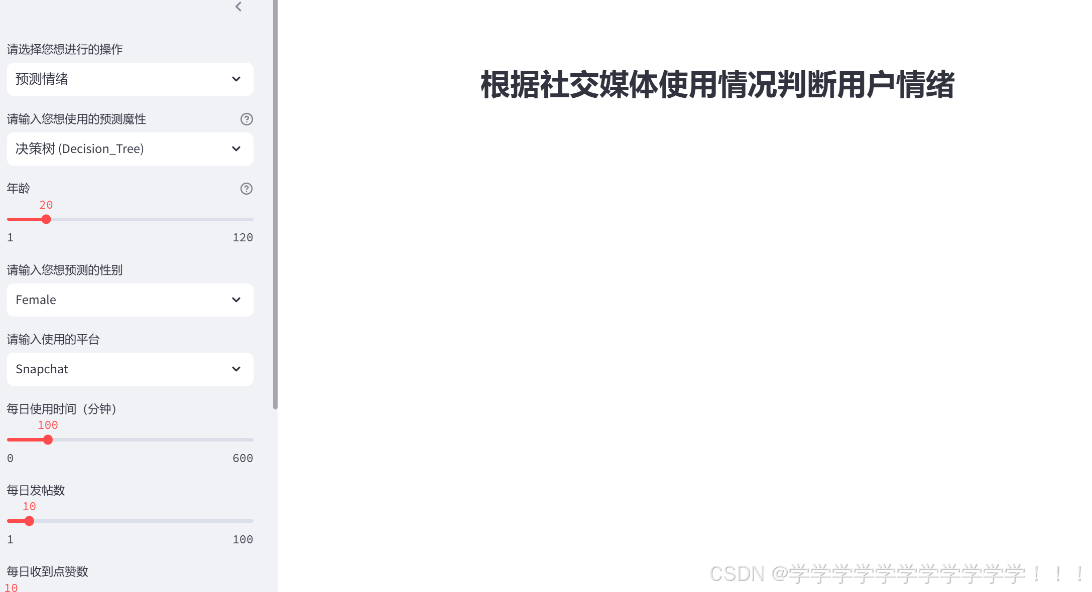
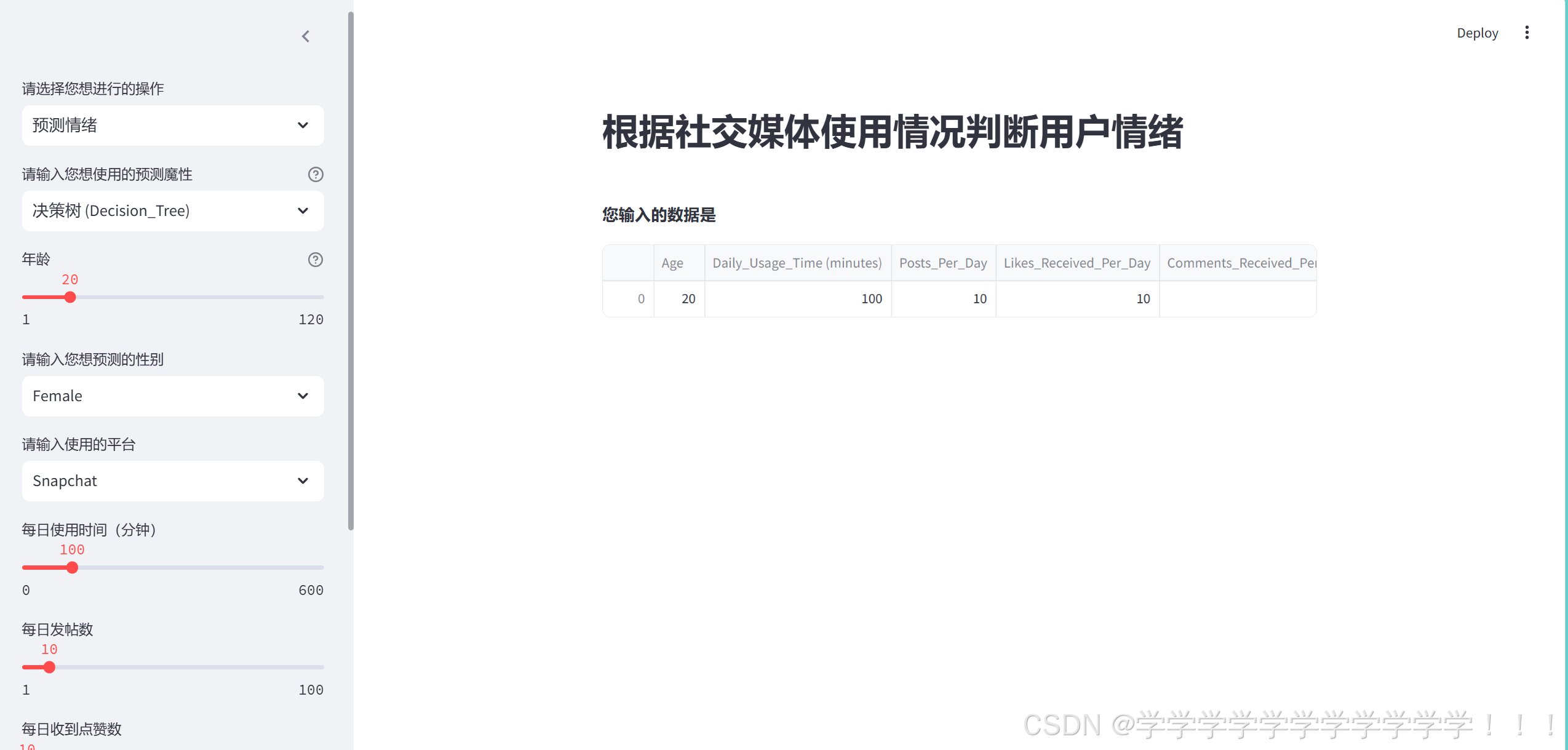
    d = pd.DataFrame([user_data], columns=features)
    if d.loc[0, "Gender"] == 'Male':
        d["Gender_Male"] = [1]
    else:
        d["Gender_Non-binary"] = [1]
    d["Platform" + "_" + str(d.loc[0, "Platform"])] = [1]
    d.drop("Platform", axis=1)
    d.drop("Gender", axis=1)

    missing_cols_test = set(test_x.columns) - set(d.columns)
    for col in missing_cols_test:
        d[col] = 0
    d = d[test_x.columns]
    y_pred_model = model_pred.predict(test_x)
    model_accuracy = accuracy_score(test_y, y_pred_model)
    pred = model_pred.predict(d)[0]
    st.markdown('')
    st.markdown('')
    st.markdown(f'''

        **您输入的数据是**
        ''')
    st.write(d)
这里将用户传入的数据放进pandas里,并对数据进行编码,方便后边进行预测
编码后的数据是
,Age,Daily_Usage_Time (minutes),Posts_Per_Day,Likes_Received_Per_Day,Comments_Received_Per_Day,Messages_Sent_Per_Day,Gender_Male,Gender_Non-binary,Platform_Instagram,Platform_LinkedIn,Platform_Snapchat,Platform_Telegram,Platform_Twitter,Platform_Whatsapp
0,20,100,10,10,10,10,0,1,0,0,1,0,0,0
下面可以进行预测和画图
    model_accuracy = model_accuracy*100
    model_accuracy = int(model_accuracy)
    model_accuracy = model_accuracy/100
    # st.markdown(f'''
    # **您预测的情绪是**
    # # {pred}
    # **准确率为{model_accuracy*100}%**
    #
    # ''')
    progress_bar = st.sidebar.progress(0)
    status_text = st.sidebar.empty()
    last_rows = np.random.randn(1, 1)
    # st.write(last_rows)
    chart = st.line_chart(last_rows, x_label="迭代次数", y_label="模型综合成绩")

    # 定义指数衰减相关参数,可根据实际情况调整衰减速度等
    decay_rate = 0.0423  # 衰减率,控制系数减小的速度
    initial_coefficient = 1.07  # 初始系数,可调整初始上升幅度
    a = 20
    for i in range(1, 100):
        # 根据指数衰减公式计算基础上升幅度的系数
        base_coefficient = initial_coefficient * np.exp(-decay_rate * i)
        # 先保证有一个基础的上升趋势,取绝对值并乘以系数
        positive_random_increments = np.abs(np.random.randn(5, 1)) * base_coefficient
        # 再添加一个较小的有正有负的随机波动,让数据有波动变化,这里乘以一个较小系数来控制波动幅度
        fluctuation = np.random.randn(5, 1) * 0.1

        new_rows = last_rows[-1, :] + (positive_random_increments + fluctuation).cumsum(axis=0)
        status_text.text(f"{i}% complete")
        chart.add_rows(new_rows)
        progress_bar.progress(i)
        last_rows = new_rows
        time.sleep(0.05)
    if last_rows[-1, 0] > 98:
        last_rows[-1, 0] = 98.23
    st.markdown(f'''
            **预测准确率为{(int(last_rows[-1, 0]*100))/100}%**
            ''')
    st.markdown(f'''
    **预测的情绪是**
    # {pred}
    ''')
上面这几行是为了画一个动态的曲线图,这个图我是真服了,真是给我画累死了,硬生生画一天,一开始我想把这个图画成从0到1的范围内,表示模型的迭代过程,按照这个思路画了一两个小时后发现这简直是异想天开,因为sklearn里没有上面东西可以表示这个模型进行到哪一步了.于是我转变思路,想着我直接画一个x**(1/3)的曲线不就完了,结果这个streamlit的更新图像函数(.add_rows())不能直接添加数,又试了三四个小时发现只能添加类似np.random.randn(1, 1)格式的.
我想行吧,那就这么写,但是新问题又出现了,np.random生成的是一个随机的数,不能控制他变为我想要的曲线,最后上网查,又是问ai,最后看可以用衰减公式,当i越来越大时上升的趋势衰减的就越厉害,我想这下总算可以了把.结果你猜怎么着,从0直接涨到一千多了,又是几个小时的调试,最后才达成了这个效果,虽然还有很大的概率超过一百,当也能稳定再95左右....最后的结果是这样的,我还是比较满意的.
5.完整代码
5.1streamlit代码(st.py)
# 写前端用的库streamlit
import streamlit as st
# 导入pandas 和 numpy 用这两个库进行数据处理
import pandas as pd
import numpy as np
# 将用来画动态图
import time
# mpl将plt画的图设置中文
import matplotlib as mpl
# 用sns画图,看看最开始的数据长什么样
import seaborn as sns
# PCA将数据降维
from sklearn.decomposition import PCA
# 混淆矩阵
from sklearn.metrics import confusion_matrix
# 决策树
from sklearn.tree import DecisionTreeClassifier
# 用于画出整个决策树
from sklearn.tree import export_graphviz
import graphviz
# k-nn(k-近邻)
from sklearn.neighbors import KNeighborsClassifier
# 支持向量机
from sklearn.svm import SVC
# 集成学习
from sklearn.ensemble import BaggingClassifier
# 保存模型
import joblib
# 各种评价标准
from sklearn.metrics import accuracy_score
from sklearn.metrics import precision_score
from sklearn.metrics import recall_score
from sklearn.metrics import f1_score
# 用来画图
import matplotlib.pyplot as plt
# 将plt画出来的图设置为中文简体
mpl.rcParams['font.family'] = 'SimHei'
# 读取数据集
test_x = pd.read_csv(r"D:\social-media-usage-and-emotional-well-being\pythonProject\Data preprocessing\test_x.csv")
test_y = pd.read_csv(r"D:\social-media-usage-and-emotional-well-being\pythonProject\Data preprocessing\test_y.csv")
train_y = pd.read_csv(r"D:\social-media-usage-and-emotional-well-being\pythonProject\Data preprocessing\train_y.csv")
train_x = pd.read_csv(r"D:\social-media-usage-and-emotional-well-being\pythonProject\Data preprocessing\train_x.csv")
st.header("根据社交媒体使用情况判断用户情绪")
choice = st.sidebar.selectbox(
label='请选择您想进行的操作',
options=('预测情绪', '调试模型'),
index=0,
format_func=str,
)
if choice == '调试模型':
st.sidebar.subheader('模型选择与调参')
model = st.sidebar.selectbox(
label='请选择您想使用的模型',
options=('决策树 (Decision_Tree)', 'k-近邻 (knn)', '支持向量机 (SVM)', '集成学习 (Ensemble Learning)'),
index=0,
format_func=str,
help='目前只提供这四种模型'
)
if model == '决策树 (Decision_Tree)':
st.subheader('决策树')
iterations = st.sidebar.slider("max_depth(最大深度)", 1, 30, 20, 1, help='决策树的最大深度,限制树的生长,防止过拟合.')
min_samples_split1 = st.sidebar.slider("min_samples_split(最小分裂样本数)", 2, 50, 2, 1, help='内部节点再划分所需的最小样本数。')
min_samples_leaf1 = st.sidebar.slider("min_samples_leaf(最小叶子节点样本数)", 1, 50, 1, 1, help='叶节点所需的最小样本数。')
progress_bar = st.empty()
with st.spinner('加载中...'):
time.sleep(0.5)
# 实例决策树
Decision_Tree = DecisionTreeClassifier(criterion='entropy', max_depth=iterations, min_samples_split=min_samples_split1, min_samples_leaf=min_samples_leaf1, random_state=2024)
# 训练决策树
Decision_Tree.fit(train_x, train_y)
joblib.dump(Decision_Tree,
'D:\social-media-usage-and-emotional-well-being\pythonProject\models\Decision_Tree_model.pickle')
# 预测
Decision_Tree_pred = Decision_Tree.predict(test_x)
# precision成绩
Decision_Tree_precision = precision_score(test_y, Decision_Tree_pred, average='macro')
# recall成绩
Decision_Tree_recall = recall_score(test_y, Decision_Tree_pred, average='micro')
# f1成绩
Decision_Tree_f1 = f1_score(test_y, Decision_Tree_pred, average='weighted')
# 准确率
Decision_Tree_accuracy = accuracy_score(test_y, Decision_Tree_pred)
# 混淆矩阵
conf_matrix = confusion_matrix(test_y, Decision_Tree_pred)
# 指标名称列表
metrics = ['Accuracy', 'Precision', 'Recall', 'F1']
# 对应的指标值列表
values = [Decision_Tree_accuracy, Decision_Tree_precision, Decision_Tree_recall, Decision_Tree_f1]
# 绘制条形图
fig, ax = plt.subplots()
colors = ['lightcoral', 'lightgreen', 'lightskyblue', 'lightsalmon']
ax.bar(metrics, values, color=colors)
# 添加标题
ax.set_title("Decision Tree Metrics")
# 添加x轴标签
ax.set_xlabel("Metrics")
# 添加y轴标签
ax.set_ylabel("Values")
ax.set_ylim(0, 1)
# 显示图形
# st.pyplot(fig)
fig1, ax = plt.subplots()
sns.heatmap(conf_matrix, annot=True, fmt='d', cmap='Blues')
ax.set_xlabel('Predicted')
ax.set_ylabel('Actual')
# 将两个图放在一行
col1, col2 = st.columns(2)
with col1:
st.pyplot(fig)
with col2:
st.pyplot(fig1)
if st.button('显示整个决策树'):
with st.spinner('加载中...'):
time.sleep(0.5)
target_names = list('Age, Daily_Usage_Time(minutes), Posts_Per_Day, Likes_Received_Per_Day, Comments_Received_Per_Day, Messages_Sent_Per_Day, Gender_Male, Gender_Non - binary, Platform_Instagram, Platform_LinkedIn, Platform_Snapchat, Platform_Telegram, Platform_Twitter, Platform_Whatsapp'.split(","))
# 将决策树模型导出为graphviz格式的dot文件
dot_data = export_graphviz(Decision_Tree, out_file=None,
feature_names=target_names,
class_names=list(set(test_y['Dominant_Emotion'])),
filled=True, rounded=True,
special_characters=True)
# 使用graphviz库的Source函数将dot文件转换为可视化图形
graph = graphviz.Source(dot_data)
st.graphviz_chart(dot_data)
st.code('''
if model == '决策树 (Decision_Tree)':
st.subheader('决策树')
iterations = st.sidebar.slider("max_depth(最大深度)", 1, 30, 20, 1, help='决策树的最大深度,限制树的生长,防止过拟合.')
min_samples_split1 = st.sidebar.slider("min_samples_split(最小分裂样本数)", 2, 50, 2, 1, help='内部节点再划分所需的最小样本数。')
min_samples_leaf1 = st.sidebar.slider("min_samples_leaf(最小叶子节点样本数)", 1, 50, 1, 1, help='叶节点所需的最小样本数。')
progress_bar = st.empty()
with st.spinner('加载中...'):
time.sleep(0.5)
# 实例决策树
Decision_Tree = DecisionTreeClassifier(criterion='entropy', max_depth=iterations, min_samples_split=min_samples_split1, min_samples_leaf=min_samples_leaf1, random_state=2024)
# 训练决策树
Decision_Tree.fit(train_x, train_y)
joblib.dump(Decision_Tree,
'D:\social-media-usage-and-emotional-well-being\pythonProject\models\Decision_Tree_model.pickle')
# 预测
Decision_Tree_pred = Decision_Tree.predict(test_x)
# precision成绩
Decision_Tree_precision = precision_score(test_y, Decision_Tree_pred, average='macro')
# recall成绩
Decision_Tree_recall = recall_score(test_y, Decision_Tree_pred, average='micro')
# f1成绩
Decision_Tree_f1 = f1_score(test_y, Decision_Tree_pred, average='weighted')
# 准确率
Decision_Tree_accuracy = accuracy_score(test_y, Decision_Tree_pred)
# 混淆矩阵
conf_matrix = confusion_matrix(test_y, Decision_Tree_pred)
# 指标名称列表
metrics = ['Accuracy', 'Precision', 'Recall', 'F1']
# 对应的指标值列表
values = [Decision_Tree_accuracy, Decision_Tree_precision, Decision_Tree_recall, Decision_Tree_f1]
# 绘制条形图
fig, ax = plt.subplots()
colors = ['lightcoral', 'lightgreen', 'lightskyblue', 'lightsalmon']
ax.bar(metrics, values, color=colors)
# 添加标题
ax.set_title("Decision Tree Metrics")
# 添加x轴标签
ax.set_xlabel("Metrics")
# 添加y轴标签
ax.set_ylabel("Values")
ax.set_ylim(0, 1)
# 显示图形
# st.pyplot(fig)
fig1, ax = plt.subplots()
sns.heatmap(conf_matrix, annot=True, fmt='d', cmap='Blues')
ax.set_xlabel('Predicted')
ax.set_ylabel('Actual')
# 将两个图放在一行
col1, col2 = st.columns(2)
with col1:
st.pyplot(fig)
with col2:
st.pyplot(fig1)
if st.button('显示整个决策树'):
with st.spinner('加载中...'):
time.sleep(0.5)
target_names = list('Age, Daily_Usage_Time(minutes), Posts_Per_Day, Likes_Received_Per_Day, Comments_Received_Per_Day, Messages_Sent_Per_Day, Gender_Male, Gender_Non - binary, Platform_Instagram, Platform_LinkedIn, Platform_Snapchat, Platform_Telegram, Platform_Twitter, Platform_Whatsapp'.split(","))
# 将决策树模型导出为graphviz格式的dot文件
dot_data = export_graphviz(Decision_Tree, out_file=None,
feature_names=target_names,
class_names=list(set(test_y['Dominant_Emotion'])),
filled=True, rounded=True,
special_characters=True)
# 使用graphviz库的Source函数将dot文件转换为可视化图形
graph = graphviz.Source(dot_data)
st.graphviz_chart(dot_data)
''')
elif model == 'k-近邻 (knn)':
st.subheader('k-近邻')
n_neighbors = st.sidebar.slider("n_neighbors(k值)", 1, 100, 3, 1,
help='决策树的最大深度,限制树的生长,防止过拟合.')
weights1 = st.sidebar.selectbox(
label='weights(权重方式)',
options=('uniform(均匀权重)', 'distance(距离加权)'),
index=0,
format_func=str,
help='用于指定近邻样本的权重计算方式。'
)
if weights1 == 'uniform(均匀权重)':
weights2 = 'uniform'
else:
weights2 = 'distance'
algorithm1 = st.sidebar.selectbox(
label='algorithm(最近邻算法)',
options=('auto(自动)', 'ball_tree', 'kd_tree'),
index=0,
format_func=str,
help='用于指定计算最近邻居的算法'
)
if algorithm1 == 'auto(自动)':
algorithm1 = 'auto'
p1 = st.sidebar.selectbox(
label='距离度量方式',
options=('欧几里得距离', '曼哈顿距离'),
index=0,
format_func=str,
help='用于闵可夫斯基距离(metric = "minkowski")的参数。当p = 1时,闵可夫斯基距离就是曼哈顿距离;当p = 2时,就是欧几里得距离。。'
)
if p1 == '曼哈顿距离':
p2 = 1
else:
p2 = 2
leaf_size1 = st.sidebar.slider("leaf_size(叶子节点大小)", 1, 1000, 3, 1, help='这主要是用于 “ball_tree” 和 “kd_tree” 算法中的一个参数,它控制树的叶子节点大小。')
progress_bar = st.empty()
with st.spinner('加载中...'):
time.sleep(0.5)
knn = KNeighborsClassifier(n_neighbors=n_neighbors, weights=weights2, algorithm=algorithm1, p=p2, leaf_size=leaf_size1)
knn.fit(train_x, train_y)
joblib.dump(knn,
'D:\social-media-usage-and-emotional-well-being\pythonProject\models\knn_model.pickle')
# 预测
knn_pred = knn.predict(test_x)
# 各种成绩
knn_precision = precision_score(test_y, knn_pred, average='macro')
knn_recall = recall_score(test_y, knn_pred, average='micro')
knn_f1 = f1_score(test_y, knn_pred, average='weighted')
knn_accuracy = accuracy_score(test_y, knn_pred)
metrics = ['Accuracy', 'Precision', 'Recall', 'F1']
# 对应的指标值列表
values = [knn_accuracy, knn_precision, knn_recall, knn_f1]
# 绘制条形图
fig, ax = plt.subplots()
colors = ['lightgreen', 'lightsalmon', 'lightskyblue', 'lightcoral', ]
ax.bar(metrics, values, color=colors)
# 添加标题
ax.set_title("Decision Tree Metrics")
# 添加x轴标签
ax.set_xlabel("Metrics")
# 添加y轴标签
ax.set_ylabel("Values")
ax.set_ylim(0, 1)
# 显示图形
# st.pyplot(fig)
pca = PCA(n_components=2)
newData = pca.fit_transform(test_x)
# st.write(newData[:, 0])
colors1 = []
for i in knn_pred:
if i == 'Neutral':
colors1.append('aquamarine')
elif i == 'Anxiety':
colors1.append('chartreuse')
elif i == 'Happiness':
colors1.append('coral')
elif i == 'Boredom':
colors1.append('dodgerblue')
elif i == 'Sadness':
colors1.append('firebrick')
elif i == 'Anger':
colors1.append('orchid')
fig3, ax = plt.subplots()
ax.scatter(newData[:, 0], newData[:, 1], c=colors1, s=40)
ax.set_title("K - NN Classification Visualization after PCA")
ax.set_xlabel("Principal Component 1")
ax.set_ylabel("Principal Component 2")
# st.pyplot(fig3)
col1, col2 = st.columns(2)
with col1:
st.pyplot(fig)
with col2:
st.pyplot(fig3)
st.code('''
elif model == 'k-近邻 (knn)':
st.subheader('k-近邻')
n_neighbors = st.sidebar.slider("n_neighbors(k值)", 1, 100, 3, 1,
help='决策树的最大深度,限制树的生长,防止过拟合.')
weights1 = st.sidebar.selectbox(
label='weights(权重方式)',
options=('uniform(均匀权重)', 'distance(距离加权)'),
index=0,
format_func=str,
help='用于指定近邻样本的权重计算方式。'
)
if weights1 == 'uniform(均匀权重)':
weights2 = 'uniform'
else:
weights2 = 'distance'
algorithm1 = st.sidebar.selectbox(
label='algorithm(最近邻算法)',
options=('auto(自动)', 'ball_tree', 'kd_tree'),
index=0,
format_func=str,
help='用于指定计算最近邻居的算法'
)
if algorithm1 == 'auto(自动)':
algorithm1 = 'auto'
p1 = st.sidebar.selectbox(
label='距离度量方式',
options=('欧几里得距离', '曼哈顿距离'),
index=0,
format_func=str,
help='用于闵可夫斯基距离(metric = "minkowski")的参数。当p = 1时,闵可夫斯基距离就是曼哈顿距离;当p = 2时,就是欧几里得距离。。'
)
if p1 == '曼哈顿距离':
p2 = 1
else:
p2 = 2
leaf_size1 = st.sidebar.slider("leaf_size(叶子节点大小)", 1, 1000, 3, 1, help='这主要是用于 “ball_tree” 和 “kd_tree” 算法中的一个参数,它控制树的叶子节点大小。')
progress_bar = st.empty()
with st.spinner('加载中...'):
time.sleep(0.5)
knn = KNeighborsClassifier(n_neighbors=n_neighbors, weights=weights2, algorithm=algorithm1, p=p2, leaf_size=leaf_size1)
knn.fit(train_x, train_y)
joblib.dump(knn,
'D:\social-media-usage-and-emotional-well-being\pythonProject\models\knn_model.pickle')
# 预测
knn_pred = knn.predict(test_x)
# 各种成绩
knn_precision = precision_score(test_y, knn_pred, average='macro')
knn_recall = recall_score(test_y, knn_pred, average='micro')
knn_f1 = f1_score(test_y, knn_pred, average='weighted')
knn_accuracy = accuracy_score(test_y, knn_pred)
metrics = ['Accuracy', 'Precision', 'Recall', 'F1']
# 对应的指标值列表
values = [knn_accuracy, knn_precision, knn_recall, knn_f1]
# 绘制条形图
fig, ax = plt.subplots()
colors = ['lightgreen', 'lightsalmon', 'lightskyblue', 'lightcoral', ]
ax.bar(metrics, values, color=colors)
# 添加标题
ax.set_title("Decision Tree Metrics")
# 添加x轴标签
ax.set_xlabel("Metrics")
# 添加y轴标签
ax.set_ylabel("Values")
ax.set_ylim(0, 1)
# 显示图形
# st.pyplot(fig)
pca = PCA(n_components=2)
newData = pca.fit_transform(test_x)
# st.write(newData[:, 0])
colors1 = []
for i in knn_pred:
if i == 'Neutral':
colors1.append('aquamarine')
elif i == 'Anxiety':
colors1.append('chartreuse')
elif i == 'Happiness':
colors1.append('coral')
elif i == 'Boredom':
colors1.append('dodgerblue')
elif i == 'Sadness':
colors1.append('firebrick')
elif i == 'Anger':
colors1.append('orchid')
fig3, ax = plt.subplots()
ax.scatter(newData[:, 0], newData[:, 1], c=colors1, s=40)
ax.set_title("K - NN Classification Visualization after PCA")
ax.set_xlabel("Principal Component 1")
ax.set_ylabel("Principal Component 2")
# st.pyplot(fig3)
col1, col2 = st.columns(2)
with col1:
st.pyplot(fig)
with col2:
st.pyplot(fig3)
''')
elif model == '支持向量机 (SVM)':
st.subheader('支持向量机')
kernel = st.sidebar.selectbox(
label='kernel(核函数类型)',
options=('rbf(径向基函数核)', 'linear(线性核)', 'polynomial(多项式核)'),
index=0,
format_func=str,
help='核函数类型'
)
if kernel == 'rbf(径向基函数核)':
kernel = 'rbf'
c = st.sidebar.slider("C(惩罚参数)", 1, 10000, 10000, 1,
help='控制对错误分类的惩罚程度')
elif kernel == 'linear(线性核)':
kernel = 'linear'
c = st.sidebar.slider("C(惩罚参数)", 1, 10, 1, 1,
help='控制对错误分类的惩罚程度')
else:
kernel = 'poly'
c = st.sidebar.slider("C(惩罚参数)", 1, 1000, 100, 1,
help='控制对错误分类的惩罚程度')
shrinking = st.sidebar.selectbox(
label='shrinking(是否使用收缩启发式)',
options=(True, False),
index=0,
format_func=str,
help='在训练过程中可能会改变优化算法的行为,不使用收缩启发式可能会使训练时间变长,但在某些特定情况下可能会提高模型的稳定性或者准确性。'
)
probability = st.sidebar.selectbox(
label='probability(是否启用概率估计)',
options=(True, False),
index=0,
format_func=str,
help='在训练过程中可能会改变优化算法的行为,不使用收缩启发式可能会使训练时间变长,但在某些特定情况下可能会提高模型的稳定性或者准确性。'
)
svm = SVC(C=c, kernel=kernel, gamma='scale', shrinking=shrinking, probability=probability)
svm.fit(train_x, train_y)
joblib.dump(svm,
'D:\social-media-usage-and-emotional-well-being\pythonProject\models\svm_model.pickle')
svm_pred = svm.predict(test_x)
svm_precision = precision_score(test_y, svm_pred, average='macro')
svm_recall = recall_score(test_y, svm_pred, average='micro')
svm_f1 = f1_score(test_y, svm_pred, average='weighted')
svm_accuracy = accuracy_score(test_y, svm_pred)
metrics = ['Accuracy', 'Precision', 'Recall', 'F1']
# 对应的指标值列表
values = [svm_accuracy, svm_precision, svm_recall, svm_f1]
# 绘制条形图
fig, ax = plt.subplots()
colors = ['lightgreen', 'lightsalmon', 'lightskyblue', 'lightcoral', ]
ax.bar(metrics, values, color=colors)
# 添加标题
ax.set_title("Decision Tree Metrics")
# 添加x轴标签
ax.set_xlabel("Metrics")
# 添加y轴标签
ax.set_ylabel("Values")
ax.set_ylim(0, 1)
# 显示图形
st.pyplot(fig)
if st.button('显示3D散点模型'):
with st.spinner('加载中...'):
# 创建PCA对象,指定降维到3个主成分
pca = PCA(n_components=3)
# 对训练集和测试集都执行降维操作
train_x_pca = pca.fit_transform(train_x)
test_x_pca = pca.transform(test_x)
# 创建三维坐标轴对象
fig1 = plt.figure(figsize=(10, 8))
# 修改此处,确保使用正确的图形对象来添加坐标轴
ax = fig1.add_subplot(111, projection='3d')
# 获取不同类别对应的索引
unique_classes = np.unique(train_y)
colors = ['r', 'g', 'b'] # 为不同类别设置不同颜色
# 绘制训练集数据点
for class_idx, color in zip(unique_classes, colors):
class_mask = train_y == class_idx
# 这里修改索引方式,通过循环每个样本进行正确索引
for sample_idx in np.where(class_mask)[0]:
ax.scatter(train_x_pca[sample_idx, 0], train_x_pca[sample_idx, 1], train_x_pca[sample_idx, 2],
c=color)
# 绘制测试集数据点(可选择以不同样式展示,比如用空心圆等,便于区分训练集和测试集)
for class_idx, color in zip(unique_classes, colors):
class_mask = test_y == class_idx
for sample_idx in np.where(class_mask)[0]:
ax.scatter(test_x_pca[sample_idx, 0], test_x_pca[sample_idx, 1], test_x_pca[sample_idx, 2],
c=color, marker='o', facecolors='none', edgecolors=color )
# 设置坐标轴标签
ax.set_xlabel('Principal Component 1')
ax.set_ylabel('Principal Component 2')
ax.set_zlabel('Principal Component 3')
ax.set_title('SVM Classification Visualization in 3D (After PCA)')
ax.legend()
# 在Streamlit中展示图形
st.pyplot(fig1)
st.code('''
elif model == '支持向量机 (SVM)':
st.subheader('支持向量机')
kernel = st.sidebar.selectbox(
label='kernel(核函数类型)',
options=('rbf(径向基函数核)', 'linear(线性核)', 'polynomial(多项式核)'),
index=0,
format_func=str,
help='核函数类型'
)
if kernel == 'rbf(径向基函数核)':
kernel = 'rbf'
c = st.sidebar.slider("C(惩罚参数)", 1, 10000, 10000, 1,
help='控制对错误分类的惩罚程度')
elif kernel == 'linear(线性核)':
kernel = 'linear'
c = st.sidebar.slider("C(惩罚参数)", 1, 10, 1, 1,
help='控制对错误分类的惩罚程度')
else:
kernel = 'poly'
c = st.sidebar.slider("C(惩罚参数)", 1, 1000, 100, 1,
help='控制对错误分类的惩罚程度')
shrinking = st.sidebar.selectbox(
label='shrinking(是否使用收缩启发式)',
options=(True, False),
index=0,
format_func=str,
help='在训练过程中可能会改变优化算法的行为,不使用收缩启发式可能会使训练时间变长,但在某些特定情况下可能会提高模型的稳定性或者准确性。'
)
probability = st.sidebar.selectbox(
label='probability(是否启用概率估计)',
options=(True, False),
index=0,
format_func=str,
help='在训练过程中可能会改变优化算法的行为,不使用收缩启发式可能会使训练时间变长,但在某些特定情况下可能会提高模型的稳定性或者准确性。'
)
svm = SVC(C=c, kernel=kernel, gamma='scale', shrinking=shrinking, probability=probability)
svm.fit(train_x, train_y)
joblib.dump(svm,
'D:\social-media-usage-and-emotional-well-being\pythonProject\models\svm_model.pickle')
svm_pred = svm.predict(test_x)
svm_precision = precision_score(test_y, svm_pred, average='macro')
svm_recall = recall_score(test_y, svm_pred, average='micro')
svm_f1 = f1_score(test_y, svm_pred, average='weighted')
svm_accuracy = accuracy_score(test_y, svm_pred)
metrics = ['Accuracy', 'Precision', 'Recall', 'F1']
# 对应的指标值列表
values = [svm_accuracy, svm_precision, svm_recall, svm_f1]
# 绘制条形图
fig, ax = plt.subplots()
colors = ['lightgreen', 'lightsalmon', 'lightskyblue', 'lightcoral', ]
ax.bar(metrics, values, color=colors)
# 添加标题
ax.set_title("Decision Tree Metrics")
# 添加x轴标签
ax.set_xlabel("Metrics")
# 添加y轴标签
ax.set_ylabel("Values")
ax.set_ylim(0, 1)
# 显示图形
st.pyplot(fig)
if st.button('显示3D散点模型'):
with st.spinner('加载中...'):
# 创建PCA对象,指定降维到3个主成分
pca = PCA(n_components=3)
# 对训练集和测试集都执行降维操作
train_x_pca = pca.fit_transform(train_x)
test_x_pca = pca.transform(test_x)
# 创建三维坐标轴对象
fig1 = plt.figure(figsize=(10, 8))
# 修改此处,确保使用正确的图形对象来添加坐标轴
ax = fig1.add_subplot(111, projection='3d')
# 获取不同类别对应的索引
unique_classes = np.unique(train_y)
colors = ['r', 'g', 'b'] # 为不同类别设置不同颜色
# 绘制训练集数据点
for class_idx, color in zip(unique_classes, colors):
class_mask = train_y == class_idx
# 这里修改索引方式,通过循环每个样本进行正确索引
for sample_idx in np.where(class_mask)[0]:
ax.scatter(train_x_pca[sample_idx, 0], train_x_pca[sample_idx, 1], train_x_pca[sample_idx, 2],
c=color)
# 绘制测试集数据点(可选择以不同样式展示,比如用空心圆等,便于区分训练集和测试集)
for class_idx, color in zip(unique_classes, colors):
class_mask = test_y == class_idx
for sample_idx in np.where(class_mask)[0]:
ax.scatter(test_x_pca[sample_idx, 0], test_x_pca[sample_idx, 1], test_x_pca[sample_idx, 2],
c=color, marker='o', facecolors='none', edgecolors=color )
# 设置坐标轴标签
ax.set_xlabel('Principal Component 1')
ax.set_ylabel('Principal Component 2')
ax.set_zlabel('Principal Component 3')
ax.set_title('SVM Classification Visualization in 3D (After PCA)')
ax.legend()
# 在Streamlit中展示图形
st.pyplot(fig1)
''')
elif model == '集成学习 (Ensemble Learning)':
st.subheader("集成学习")
st.sidebar.subheader('基础学习器')
base_model = st.sidebar.selectbox(
label='选择基础学习器',
options=('Decision_Tree', 'knn'),
index=0,
format_func=str,
help='在训练过程中可能会改变优化算法的行为,不使用收缩启发式可能会使训练时间变长,但在某些特定情况下可能会提高模型的稳定性或者准确性。'
)
#决策树
if base_model=="Decision_Tree":
iterations = st.sidebar.slider("max_depth(最大深度)", 1, 30, 20, 1,
help='决策树的最大深度,限制树的生长,防止过拟合.')
min_samples_split1 = st.sidebar.slider("min_samples_split(最小分裂样本数)", 2, 50, 2, 1,
help='内部节点再划分所需的最小样本数。')
min_samples_leaf1 = st.sidebar.slider("min_samples_leaf(最小叶子节点样本数)", 1, 50, 1, 1,
help='叶节点所需的最小样本数。')
base_clf = DecisionTreeClassifier(criterion='entropy', max_depth=iterations,
min_samples_split=min_samples_split1, min_samples_leaf=min_samples_leaf1,
random_state=2024)
base_clf.fit(train_x, train_y)
joblib.dump(base_clf,
r'D:\social-media-usage-and-emotional-well-being\pythonProject\models\base_clf.pickle')
else:
n_neighbors = st.sidebar.slider("n_neighbors(k值)", 1, 100, 3, 1,
help='决策树的最大深度,限制树的生长,防止过拟合.')
weights1 = st.sidebar.selectbox(
label='weights(权重方式)',
options=('uniform(均匀权重)', 'distance(距离加权)'),
index=0,
format_func=str,
help='用于指定近邻样本的权重计算方式。'
)
if weights1 == 'uniform(均匀权重)':
weights2 = 'uniform'
else:
weights2 = 'distance'
algorithm1 = st.sidebar.selectbox(
label='algorithm(最近邻算法)',
options=('auto(自动)', 'ball_tree', 'kd_tree'),
index=0,
format_func=str,
help='用于指定计算最近邻居的算法'
)
if algorithm1 == 'auto(自动)':
algorithm1 = 'auto'
p1 = st.sidebar.selectbox(
label='距离度量方式',
options=('欧几里得距离', '曼哈顿距离'),
index=0,
format_func=str,
help='用于闵可夫斯基距离(metric = "minkowski")的参数。当p = 1时,闵可夫斯基距离就是曼哈顿距离;当p = 2时,就是欧几里得距离。。'
)
if p1 == '曼哈顿距离':
p2 = 1
else:
p2 = 2
leaf_size1 = st.sidebar.slider("leaf_size(叶子节点大小)", 1, 1000, 3, 1,
help='这主要是用于 “ball_tree” 和 “kd_tree” 算法中的一个参数,它控制树的叶子节点大小。')
base_clf = KNeighborsClassifier(n_neighbors=n_neighbors, weights=weights2, algorithm=algorithm1, p=p2, leaf_size=leaf_size1)
base_clf.fit(train_x, train_y)
joblib.dump(base_clf,
r'D:\social-media-usage-and-emotional-well-being\pythonProject\models\base_clf.pickle')
pca = PCA(n_components=2)
newData = pca.fit_transform(test_x)
st.sidebar.subheader('集成分类器')
n_estimators = st.sidebar.slider("n_estimators(基学习器的数量)", 1, 30, 10, 1,
help='这个参数是可以调整的重要参数。它决定了集成学习中基学习器(例如决策树)的数量。增加n_estimators通常可以提高模型的性能和稳定性,但也会增加计算成本和训练时间。例如,当处理一个复杂的分类问题,数据有较多的噪声和特征时,适当增加n_estimators可能会使模型更好地拟合数据。')
max_samples = st.sidebar.slider("max_samples(抽样的样本比例)", 0.0, 1.0, 1.0, format="%.2f",
help='用于控制每次构建基学习器时从训练数据集中抽样的样本比例(如果值小于 1.0)或样本数量(如果值为整数)。调整这个参数可以改变基学习器训练数据的多样性。如果数据量很大,适当减小max_samples可以减少每个基学习器的训练时间,同时增加基学习器之间的差异。')
max_features = st.sidebar.slider("max_samples(抽样的样本比例)", 0.0, 1.0, 1.0, format="%.2f",
help='控制每次构建基学习器时从特征集合中抽取的特征比例(如果值小于 1.0)或特征数量(如果值为整数)。通过调整这个参数可以引入特征的随机性,特别是在特征维度较高的情况下,能够防止模型过度依赖某些特征,提高模型的泛化能力。')
bootstrap = st.sidebar.selectbox(
label='bootstrap(是否采用有放回基学习器)',
options=(True, False),
index=0,
format_func=str,
help='在训练过程中可能会改变优化算法的行为,不使用收缩启发式可能会使训练时间变长,但在某些特定情况下可能会提高模型的稳定性或者准确性。'
)
bootstrap_features = st.sidebar.selectbox(
label='bootstrap(是否采用有放回特征)',
options=(True, False),
index=0,
format_func=str,
help='在训练过程中可能会改变优化算法的行为,不使用收缩启发式可能会使训练时间变长,但在某些特定情况下可能会提高模型的稳定性或者准确性。'
)
with st.spinner('加载中...'):
time.sleep(0.5)
bagging_clf = BaggingClassifier(base_clf, n_estimators=n_estimators, max_samples=max_samples, max_features=max_features, bootstrap=bootstrap, bootstrap_features=bootstrap_features, random_state=42)
bagging_clf.fit(train_x, train_y)
joblib.dump(bagging_clf,
r'D:\social-media-usage-and-emotional-well-being\pythonProject\models\bagging_clf.pickle')
# 训练基础分类器模型
y_pred_base_clf = base_clf.predict(test_x)
y_pred_bagging = bagging_clf.predict(test_x)
bagging_clf_precision = precision_score(test_y, y_pred_bagging, average='macro')
bagging_clf_recall = recall_score(test_y, y_pred_bagging, average='micro')
bagging_clf_f1 = f1_score(test_y, y_pred_bagging, average='weighted')
bagging_clf_accuracy = accuracy_score(test_y, y_pred_bagging)
metrics = ['Accuracy', 'Precision', 'Recall', 'F1']
# 对应的指标值列表
values = [bagging_clf_accuracy, bagging_clf_precision, bagging_clf_recall, bagging_clf_f1]
# 绘制条形图
fig, ax = plt.subplots()
colors = ['lightgreen', 'lightsalmon', 'lightskyblue', 'lightcoral' ]
ax.bar(metrics, values, color=colors)
# 添加标题
ax.set_title("集成学习器")
# 添加x轴标签
ax.set_xlabel("Metrics")
# 添加y轴标签
ax.set_ylabel("Values")
ax.set_ylim(0, 1)
# 显示图形
# st.pyplot(fig)
base_clf_precision = precision_score(test_y, y_pred_base_clf, average='macro')
base_clf_recall = recall_score(test_y, y_pred_base_clf, average='micro')
base_clf_f1 = f1_score(test_y, y_pred_base_clf, average='weighted')
base_clf_accuracy = accuracy_score(test_y, y_pred_base_clf)
metrics = ['Accuracy', 'Precision', 'Recall', 'F1']
# 对应的指标值列表
values = [base_clf_accuracy, base_clf_precision, base_clf_recall, base_clf_f1]
# 绘制条形图
fig1, ax = plt.subplots()
colors = ['lightgreen', 'lightsalmon', 'lightskyblue', 'lightcoral']
ax.bar(metrics, values, color=colors)
# 添加标题
ax.set_title("基础学习器")
# 添加x轴标签
ax.set_xlabel("Metrics")
# 添加y轴标签
ax.set_ylabel("Values")
ax.set_ylim(0, 1)
# 显示图形
# st.pyplot(fig)
col1, col2 = st.columns(2)
with col1:
st.pyplot(fig)
with col2:
st.pyplot(fig1)
if base_model == "Decision_Tree":
cb = st.checkbox('显示决策树', value=False)
if cb:
with st.spinner('加载中...'):
time.sleep(0.5)
target_names = list(
'Age, Daily_Usage_Time(minutes), Posts_Per_Day, Likes_Received_Per_Day, Comments_Received_Per_Day, Messages_Sent_Per_Day, Gender_Male, Gender_Non - binary, Platform_Instagram, Platform_LinkedIn, Platform_Snapchat, Platform_Telegram, Platform_Twitter, Platform_Whatsapp'.split(
","))
# 将决策树模型导出为graphviz格式的dot文件
dot_data = export_graphviz(base_clf, out_file=None,
feature_names=target_names,
class_names=list(set(test_y['Dominant_Emotion'])),
filled=True, rounded=True,
special_characters=True)
# 使用graphviz库的Source函数将dot文件转换为可视化图形
graph = graphviz.Source(dot_data)
st.graphviz_chart(dot_data)
else:
# st.write(newData[:, 0])
cb1 = st.checkbox('显示knn', value=False)
if cb1:
colors1 = []
for i in y_pred_base_clf:
if i == 'Neutral':
colors1.append('aquamarine')
elif i == 'Anxiety':
colors1.append('chartreuse')
elif i == 'Happiness':
colors1.append('coral')
elif i == 'Boredom':
colors1.append('dodgerblue')
elif i == 'Sadness':
colors1.append('firebrick')
elif i == 'Anger':
colors1.append('orchid')
pca = PCA(n_components=2)
newData = pca.fit_transform(test_x)
fig3, ax = plt.subplots()
ax.scatter(newData[:, 0], newData[:, 1], c=colors1, s=40)
ax.set_title("K - NN Classification Visualization after PCA")
ax.set_xlabel("Principal Component 1")
ax.set_ylabel("Principal Component 2")
st.pyplot(fig3)
st.code('''
elif model == '集成学习 (Ensemble Learning)':
st.subheader("集成学习")
st.sidebar.subheader('基础学习器')
base_model = st.sidebar.selectbox(
label='选择基础学习器',
options=('Decision_Tree', 'knn'),
index=0,
format_func=str,
help='在训练过程中可能会改变优化算法的行为,不使用收缩启发式可能会使训练时间变长,但在某些特定情况下可能会提高模型的稳定性或者准确性。'
)
#决策树
if base_model=="Decision_Tree":
iterations = st.sidebar.slider("max_depth(最大深度)", 1, 30, 20, 1,
help='决策树的最大深度,限制树的生长,防止过拟合.')
min_samples_split1 = st.sidebar.slider("min_samples_split(最小分裂样本数)", 2, 50, 2, 1,
help='内部节点再划分所需的最小样本数。')
min_samples_leaf1 = st.sidebar.slider("min_samples_leaf(最小叶子节点样本数)", 1, 50, 1, 1,
help='叶节点所需的最小样本数。')
base_clf = DecisionTreeClassifier(criterion='entropy', max_depth=iterations,
min_samples_split=min_samples_split1, min_samples_leaf=min_samples_leaf1,
random_state=2024)
base_clf.fit(train_x, train_y)
joblib.dump(base_clf,
r'D:\social-media-usage-and-emotional-well-being\pythonProject\models\base_clf.pickle')
else:
n_neighbors = st.sidebar.slider("n_neighbors(k值)", 1, 100, 3, 1,
help='决策树的最大深度,限制树的生长,防止过拟合.')
weights1 = st.sidebar.selectbox(
label='weights(权重方式)',
options=('uniform(均匀权重)', 'distance(距离加权)'),
index=0,
format_func=str,
help='用于指定近邻样本的权重计算方式。'
)
if weights1 == 'uniform(均匀权重)':
weights2 = 'uniform'
else:
weights2 = 'distance'
algorithm1 = st.sidebar.selectbox(
label='algorithm(最近邻算法)',
options=('auto(自动)', 'ball_tree', 'kd_tree'),
index=0,
format_func=str,
help='用于指定计算最近邻居的算法'
)
if algorithm1 == 'auto(自动)':
algorithm1 = 'auto'
p1 = st.sidebar.selectbox(
label='距离度量方式',
options=('欧几里得距离', '曼哈顿距离'),
index=0,
format_func=str,
help='用于闵可夫斯基距离(metric = "minkowski")的参数。当p = 1时,闵可夫斯基距离就是曼哈顿距离;当p = 2时,就是欧几里得距离。。'
)
if p1 == '曼哈顿距离':
p2 = 1
else:
p2 = 2
leaf_size1 = st.sidebar.slider("leaf_size(叶子节点大小)", 1, 1000, 3, 1,
help='这主要是用于 “ball_tree” 和 “kd_tree” 算法中的一个参数,它控制树的叶子节点大小。')
base_clf = KNeighborsClassifier(n_neighbors=n_neighbors, weights=weights2, algorithm=algorithm1, p=p2, leaf_size=leaf_size1)
base_clf.fit(train_x, train_y)
joblib.dump(base_clf,
r'D:\social-media-usage-and-emotional-well-being\pythonProject\models\base_clf.pickle')
pca = PCA(n_components=2)
newData = pca.fit_transform(test_x)
st.sidebar.subheader('集成分类器')
n_estimators = st.sidebar.slider("n_estimators(基学习器的数量)", 1, 30, 10, 1,
help='这个参数是可以调整的重要参数。它决定了集成学习中基学习器(例如决策树)的数量。增加n_estimators通常可以提高模型的性能和稳定性,但也会增加计算成本和训练时间。例如,当处理一个复杂的分类问题,数据有较多的噪声和特征时,适当增加n_estimators可能会使模型更好地拟合数据。')
max_samples = st.sidebar.slider("max_samples(抽样的样本比例)", 0.0, 1.0, 1.0, format="%.2f",
help='用于控制每次构建基学习器时从训练数据集中抽样的样本比例(如果值小于 1.0)或样本数量(如果值为整数)。调整这个参数可以改变基学习器训练数据的多样性。如果数据量很大,适当减小max_samples可以减少每个基学习器的训练时间,同时增加基学习器之间的差异。')
max_features = st.sidebar.slider("max_samples(抽样的样本比例)", 0.0, 1.0, 1.0, format="%.2f",
help='控制每次构建基学习器时从特征集合中抽取的特征比例(如果值小于 1.0)或特征数量(如果值为整数)。通过调整这个参数可以引入特征的随机性,特别是在特征维度较高的情况下,能够防止模型过度依赖某些特征,提高模型的泛化能力。')
bootstrap = st.sidebar.selectbox(
label='bootstrap(是否采用有放回基学习器)',
options=(True, False),
index=0,
format_func=str,
help='在训练过程中可能会改变优化算法的行为,不使用收缩启发式可能会使训练时间变长,但在某些特定情况下可能会提高模型的稳定性或者准确性。'
)
bootstrap_features = st.sidebar.selectbox(
label='bootstrap(是否采用有放回特征)',
options=(True, False),
index=0,
format_func=str,
help='在训练过程中可能会改变优化算法的行为,不使用收缩启发式可能会使训练时间变长,但在某些特定情况下可能会提高模型的稳定性或者准确性。'
)
with st.spinner('加载中...'):
time.sleep(0.5)
bagging_clf = BaggingClassifier(base_clf, n_estimators=n_estimators, max_samples=max_samples, max_features=max_features, bootstrap=bootstrap, bootstrap_features=bootstrap_features, random_state=42)
bagging_clf.fit(train_x, train_y)
joblib.dump(bagging_clf,
r'D:\social-media-usage-and-emotional-well-being\pythonProject\models\bagging_clf.pickle')
# 训练基础分类器模型
y_pred_base_clf = base_clf.predict(test_x)
y_pred_bagging = bagging_clf.predict(test_x)
bagging_clf_precision = precision_score(test_y, y_pred_bagging, average='macro')
bagging_clf_recall = recall_score(test_y, y_pred_bagging, average='micro')
bagging_clf_f1 = f1_score(test_y, y_pred_bagging, average='weighted')
bagging_clf_accuracy = accuracy_score(test_y, y_pred_bagging)
metrics = ['Accuracy', 'Precision', 'Recall', 'F1']
# 对应的指标值列表
values = [bagging_clf_accuracy, bagging_clf_precision, bagging_clf_recall, bagging_clf_f1]
# 绘制条形图
fig, ax = plt.subplots()
colors = ['lightgreen', 'lightsalmon', 'lightskyblue', 'lightcoral' ]
ax.bar(metrics, values, color=colors)
# 添加标题
ax.set_title("集成学习器")
# 添加x轴标签
ax.set_xlabel("Metrics")
# 添加y轴标签
ax.set_ylabel("Values")
ax.set_ylim(0, 1)
# 显示图形
# st.pyplot(fig)
base_clf_precision = precision_score(test_y, y_pred_base_clf, average='macro')
base_clf_recall = recall_score(test_y, y_pred_base_clf, average='micro')
base_clf_f1 = f1_score(test_y, y_pred_base_clf, average='weighted')
base_clf_accuracy = accuracy_score(test_y, y_pred_base_clf)
metrics = ['Accuracy', 'Precision', 'Recall', 'F1']
# 对应的指标值列表
values = [base_clf_accuracy, base_clf_precision, base_clf_recall, base_clf_f1]
# 绘制条形图
fig1, ax = plt.subplots()
colors = ['lightgreen', 'lightsalmon', 'lightskyblue', 'lightcoral']
ax.bar(metrics, values, color=colors)
# 添加标题
ax.set_title("基础学习器")
# 添加x轴标签
ax.set_xlabel("Metrics")
# 添加y轴标签
ax.set_ylabel("Values")
ax.set_ylim(0, 1)
# 显示图形
# st.pyplot(fig)
col1, col2 = st.columns(2)
with col1:
st.pyplot(fig)
with col2:
st.pyplot(fig1)
if base_model == "Decision_Tree":
cb = st.checkbox('显示决策树', value=False)
if cb:
with st.spinner('加载中...'):
time.sleep(0.5)
target_names = list(
'Age, Daily_Usage_Time(minutes), Posts_Per_Day, Likes_Received_Per_Day, Comments_Received_Per_Day, Messages_Sent_Per_Day, Gender_Male, Gender_Non - binary, Platform_Instagram, Platform_LinkedIn, Platform_Snapchat, Platform_Telegram, Platform_Twitter, Platform_Whatsapp'.split(
","))
# 将决策树模型导出为graphviz格式的dot文件
dot_data = export_graphviz(base_clf, out_file=None,
feature_names=target_names,
class_names=list(set(test_y['Dominant_Emotion'])),
filled=True, rounded=True,
special_characters=True)
# 使用graphviz库的Source函数将dot文件转换为可视化图形
graph = graphviz.Source(dot_data)
st.graphviz_chart(dot_data)
else:
# st.write(newData[:, 0])
cb1 = st.checkbox('显示knn', value=False)
if cb1:
colors1 = []
for i in y_pred_base_clf:
if i == 'Neutral':
colors1.append('aquamarine')
elif i == 'Anxiety':
colors1.append('chartreuse')
elif i == 'Happiness':
colors1.append('coral')
elif i == 'Boredom':
colors1.append('dodgerblue')
elif i == 'Sadness':
colors1.append('firebrick')
elif i == 'Anger':
colors1.append('orchid')
pca = PCA(n_components=2)
newData = pca.fit_transform(test_x)
fig3, ax = plt.subplots()
ax.scatter(newData[:, 0], newData[:, 1], c=colors1, s=40)
ax.set_title("K - NN Classification Visualization after PCA")
ax.set_xlabel("Principal Component 1")
ax.set_ylabel("Principal Component 2")
st.pyplot(fig3)
''',language='python')
else:
# st.sidebar.subheader('集成分类器')
pred_model = st.sidebar.selectbox(
label='请输入您想使用的预测魔性',
options=('决策树 (Decision_Tree)', 'k-近邻 (knn)', '支持向量机 (SVM)', '集成学习 (Ensemble Learning)'),
index=0,
format_func=str,
help='目前只提供这四种模型'
)
if pred_model == '决策树 (Decision_Tree)':
model_pred = joblib.load(
r'D:\social-media-usage-and-emotional-well-being\pythonProject\models\Decision_Tree_model.pickle')
elif pred_model == 'k-近邻 (knn)':
model_pred = joblib.load(r'D:\social-media-usage-and-emotional-well-being\pythonProject\models\knn_model.pickle')
elif pred_model == '支持向量机 (SVM)':
model_pred = joblib.load(r'D:\social-media-usage-and-emotional-well-being\pythonProject\models\svm_model.pickle')
else:
model_pred = joblib.load(
r'D:\social-media-usage-and-emotional-well-being\pythonProject\models\bagging_clf.pickle')
age = st.sidebar.slider("年龄", 1, 120, 20, 1, help='请输入您想预测的年龄')
Gender = st.sidebar.selectbox(
label='请输入您想预测的性别',
options=('Female', 'Male','Non-binary'),
index=0,
format_func=str,
)
Platform = st.sidebar.selectbox(
label='请输入使用的平台',
options=('Snapchat', 'Telegram', 'Facebook', 'Instagram', 'Twitter', 'LinkedIn', 'Whatsapp'),
index=0,
format_func=str,
)
Daily_Usage_Time = st.sidebar.slider("每日使用时间(分钟)", 0, 600, 100, 1, key="Daily_Usage_Time的唯一键值")
Posts_Per_Day = st.sidebar.slider("每日发帖数", 1, 100, 10, 1,key="Posts_Per_Day的唯一键值")
Likes_Received_Per_Day = st.sidebar.slider("每日收到点赞数", 1, 1000, 10, 1,key="Likes_Received_Per_Day的唯一键值")
Comments_Received_Per_Day = st.sidebar.slider("每日收到评论数", 1, 1000, 10, 1,key="Comments_Received_Per_Day的唯一键值")
Messages_Sent_Per_Day = st.sidebar.slider("每日发送消息数", 1, 1000, 10, 1,key="Messages_Sent_Per_Day的唯一键值")
features = ['Age', 'Gender', 'Platform', 'Daily_Usage_Time (minutes)', 'Posts_Per_Day', 'Likes_Received_Per_Day',
'Comments_Received_Per_Day', 'Messages_Sent_Per_Day']
user_data = [age, Gender, Platform, Daily_Usage_Time, Posts_Per_Day, Likes_Received_Per_Day,
Comments_Received_Per_Day, Messages_Sent_Per_Day]
d = pd.DataFrame([user_data], columns=features)
if d.loc[0, "Gender"] == 'Male':
d["Gender_Male"] = [1]
else:
d["Gender_Non-binary"] = [1]
d["Platform" + "_" + str(d.loc[0, "Platform"])] = [1]
d.drop("Platform", axis=1)
d.drop("Gender", axis=1)
missing_cols_test = set(test_x.columns) - set(d.columns)
for col in missing_cols_test:
d[col] = 0
d = d[test_x.columns]
y_pred_model = model_pred.predict(test_x)
model_accuracy = accuracy_score(test_y, y_pred_model)
pred = model_pred.predict(d)[0]
st.markdown('')
st.markdown('')
st.markdown(f'''
**您输入的数据是**
''')
st.write(d)
model_accuracy = model_accuracy*100
model_accuracy = int(model_accuracy)
model_accuracy = model_accuracy/100
# st.markdown(f'''
# **您预测的情绪是**
# # {pred}
# **准确率为{model_accuracy*100}%**
#
# ''')
progress_bar = st.sidebar.progress(0)
status_text = st.sidebar.empty()
last_rows = np.random.randn(1, 1)
# st.write(last_rows)
chart = st.line_chart(last_rows, x_label="迭代次数", y_label="模型综合成绩")
# 定义指数衰减相关参数,可根据实际情况调整衰减速度等
decay_rate = 0.0423 # 衰减率,控制系数减小的速度
initial_coefficient = 1.07 # 初始系数,可调整初始上升幅度
a = 20
for i in range(1, 100):
# 根据指数衰减公式计算基础上升幅度的系数
base_coefficient = initial_coefficient * np.exp(-decay_rate * i)
# 先保证有一个基础的上升趋势,取绝对值并乘以系数
positive_random_increments = np.abs(np.random.randn(5, 1)) * base_coefficient
# 再添加一个较小的有正有负的随机波动,让数据有波动变化,这里乘以一个较小系数来控制波动幅度
fluctuation = np.random.randn(5, 1) * 0.1
new_rows = last_rows[-1, :] + (positive_random_increments + fluctuation).cumsum(axis=0)
status_text.text(f"{i}% complete")
chart.add_rows(new_rows)
progress_bar.progress(i)
last_rows = new_rows
time.sleep(0.05)
if last_rows[-1, 0] > 98:
last_rows[-1, 0] = 98.23
st.markdown(f'''
**预测准确率为{(int(last_rows[-1, 0]*100))/100}%**
''')
st.markdown(f'''
**预测的情绪是**
# {pred}
''')
st.code('''
# st.sidebar.subheader('集成分类器')
pred_model = st.sidebar.selectbox(
label='请输入您想使用的预测魔性',
options=('决策树 (Decision_Tree)', 'k-近邻 (knn)', '支持向量机 (SVM)', '集成学习 (Ensemble Learning)'),
index=0,
format_func=str,
help='目前只提供这四种模型'
)
if pred_model == '决策树 (Decision_Tree)':
model_pred = joblib.load(
r'D:\social-media-usage-and-emotional-well-being\pythonProject\models\Decision_Tree_model.pickle')
elif pred_model == 'k-近邻 (knn)':
model_pred = joblib.load(r'D:\social-media-usage-and-emotional-well-being\pythonProject\models\knn_model.pickle')
elif pred_model == '支持向量机 (SVM)':
model_pred = joblib.load(r'D:\social-media-usage-and-emotional-well-being\pythonProject\models\svm_model.pickle')
elif pred_model == '集成学习 (Ensemble Learning)':
model_pred = joblib.load(
r'D:\social-media-usage-and-emotional-well-being\pythonProject\models\bagging_clf.pickle')
age = st.sidebar.slider("年龄", 1, 120, 20, 1, help='请输入您想预测的年龄')
Gender = st.sidebar.selectbox(
label='请输入您想预测的性别',
options=('Female', 'Male','Non-binary'),
index=0,
format_func=str,
)
Platform = st.sidebar.selectbox(
label='请输入使用的平台',
options=('Snapchat', 'Telegram', 'Facebook', 'Instagram', 'Twitter', 'LinkedIn', 'Whatsapp'),
index=0,
format_func=str,
)
Daily_Usage_Time = st.sidebar.slider("每日使用时间(分钟)", 0, 600, 100, 1, key="Daily_Usage_Time的唯一键值")
Posts_Per_Day = st.sidebar.slider("每日发帖数", 1, 100, 10, 1,key="Posts_Per_Day的唯一键值")
Likes_Received_Per_Day = st.sidebar.slider("每日收到点赞数", 1, 1000, 10, 1,key="Likes_Received_Per_Day的唯一键值")
Comments_Received_Per_Day = st.sidebar.slider("每日收到评论数", 1, 1000, 10, 1,key="Comments_Received_Per_Day的唯一键值")
Messages_Sent_Per_Day = st.sidebar.slider("每日发送消息数", 1, 1000, 10, 1,key="Messages_Sent_Per_Day的唯一键值")
features = ['Age', 'Gender', 'Platform', 'Daily_Usage_Time (minutes)', 'Posts_Per_Day', 'Likes_Received_Per_Day',
'Comments_Received_Per_Day', 'Messages_Sent_Per_Day']
user_data = [age, Gender, Platform, Daily_Usage_Time, Posts_Per_Day, Likes_Received_Per_Day, Comments_Received_Per_Day, Messages_Sent_Per_Day]
d = pd.DataFrame([user_data], columns=features)
if d.loc[0, "Gender"] == 'Male':
d["Gender_Male"] = [1]
else:
d["Gender_Non-binary"] = [1]
d["Platform" + "_" + str(d.loc[0, "Platform"])] = [1]
d.drop("Platform", axis=1)
d.drop("Gender", axis=1)
missing_cols_test = set(test_x.columns) - set(d.columns)
for col in missing_cols_test:
d[col] = 0
d = d[test_x.columns]
y_pred_model = model_pred.predict(test_x)
model_accuracy = accuracy_score(test_y, y_pred_model)
pred = model_pred.predict(d)[0]
st.markdown('')
st.markdown('')
st.write(d)
model_accuracy = model_accuracy*100
model_accuracy = int(model_accuracy)
model_accuracy = model_accuracy/100
progress_bar = st.sidebar.progress(0)
status_text = st.sidebar.empty()
last_rows = np.random.randn(1, 1)
# st.write(last_rows)
chart = st.line_chart(last_rows,x_label="迭代次数",y_label="模型综合成绩")
# 定义指数衰减相关参数,可根据实际情况调整衰减速度等
decay_rate = 0.0423 # 衰减率,控制系数减小的速度
initial_coefficient = 1.07 # 初始系数,可调整初始上升幅度
a = 20
for i in range(1, 100):
# 根据指数衰减公式计算基础上升幅度的系数
base_coefficient = initial_coefficient * np.exp(-decay_rate * i)
# 先保证有一个基础的上升趋势,取绝对值并乘以系数
positive_random_increments = np.abs(np.random.randn(5, 1)) * base_coefficient
# 再添加一个较小的有正有负的随机波动,让数据有波动变化,这里乘以一个较小系数来控制波动幅度
fluctuation = np.random.randn(5, 1) * 0.1
new_rows = last_rows[-1, :] + (positive_random_increments + fluctuation).cumsum(axis=0)
status_text.text(f"{i}% complete")
chart.add_rows(new_rows)
progress_bar.progress(i)
last_rows = new_rows
time.sleep(0.05)
if last_rows[-1, 0] > 98:
last_rows[-1, 0] = 98.23
''',language='python')一共1302行,是我目前写的最多的一个py文件了,哈哈哈哈哈哈哈哈哈哈,其实看着还是很有成就感的
5.2html的前端和后端(/client side and server side/client.html)
html没学明白,但是改改勉强还能凑合着用,哈哈哈哈哈哈哈
<!DOCTYPE html>
<html>

<head>
  <meta charset="UTF-8">
  <meta name="viewport" content="width=device-width, initial-scale=1.0">
  <title>社交媒体用户情绪分析前端</title>

  <style>
    body {
      font-family: Arial, sans-serif;
      background-color: #f4f4f4;
    }

   .form-container {
      width: 400px;
      margin: 0 auto;
      padding: 20px;
      border: 1px solid #ccc;
      border-radius: 5px;
      box-shadow: 0 0 5px rgba(0, 0, 0, 0.1);
      background-color: white;
    }

    h1 {
      color: #333;
      text-align: center;
      margin-bottom: 20px;
    }

    label {
      display: block;
      margin-bottom: 5px;
    }

    input,
    select,
    button {
      width: 100%;
      padding: 5px;
      margin-bottom: 15px;
    }

    button {
      background-color: #007BFF;
      color: white;
      border: none;
      border-radius: 3px;
      cursor: pointer;
    }

    #result {
      margin-top: 15px;
      padding: 10px;
      border: 1px solid #ccc;
      border-radius: 3px;
    }

  </style>
</head>

<body>
  <h1>社交媒体用户情绪分析</h1>
  <div class="form-container">
    <label for="age">年龄:</label><input type="number" id="age"><br>
    <label for="gender">性别:</label><select id="gender">
      <option value="Female">Female</option>
      <option value="Male">Male</option>
      <option value="Non-binary">Non-binary</option>
    </select><br>
    <label for="platform">平台:</label><select id="platform">
      <option value="Snapchat">Snapchat</option>
      <option value="Telegram">Telegram</option>
      <option value="Facebook">Facebook</option>
      <option value="Instagram">Instagram</option>
      <option value="Twitter">Twitter</option>
      <option value="LinkedIn">LinkedIn</option>
      <option value="Whatsapp">Whatsapp</option>
    </select><br>
    <label for="usage-time">每日使用时间(分钟):</label><input type="number" id="usage-time"><br>
    <label for="posts-per-day">每日发布帖子数:</label><input type="number" id="posts-per-day"><br>
    <label for="likes-per-day">每日收到点赞数:</label><input type="number" id="likes-per-day"><br>
    <label for="comments-per-day">每日收到评论数:</label><input type="number" id="comments-per-day"><br>
    <label for="messages-per-day">每日发送消息数:</label><input type="number" id="messages-per-day"><br>
    <button onclick="predictEmotion()">预测情绪</button>
    <div id="result"></div>
  </div>

  <script>
    async function predictEmotion() {
      const age = document.getElementById('age').value;
      const gender = document.getElementById('gender').value;
      const platform = document.getElementById('platform').value;
      const usageTime = document.getElementById('usage-time').value;
      const postsPerDay = document.getElementById('posts-per-day').value;
      const likesPerDay = document.getElementById('likes-per-day').value;
      const commentsPerDay = document.getElementById('comments-per-day').value;
      const messagesPerDay = document.getElementById('messages-per-day').value;

      const userData = {
        'Age': age,
        'Gender': gender,
        'Platform': platform,
        'Daily_Usage_Time (minutes)': usageTime,
        'Posts_Per_Day': postsPerDay,
        'Likes_Received_Per_Day': likesPerDay,
        'Comments_Received_Per_Day': commentsPerDay,
        'Messages_Sent_Per_Day': messagesPerDay
      };


      // 将userData和userInput整合到一个对象中
      const combinedData = {
        userData: userData,

      };

      var xhr = new XMLHttpRequest();
      xhr.onreadystatechange = function () {
        if (this.readyState == 4 && this.status == 200) {
          var responseData = JSON.parse(this.responseText);
          document.getElementById('result').innerHTML = responseData.message;
        }
      };
      // 构造POST请求,将整合后的数据发送到后端
      xhr.open('POST', 'http://localhost:5000/api/submit', true);
      xhr.setRequestHeader('Content-Type', 'application/json');
      xhr.send(JSON.stringify(combinedData));
    }
  </script>
</body>

</html>
5.3html的前端和后端(/client side and server side/server.py)
from flask_cors import CORS  # 导入CORS
from flask import Flask, request, jsonify
import joblib
import pandas as pd

GaussianNB_model = joblib.load(r'D:\social-media-usage-and-emotional-well-being\pythonProject\models\bagging_clf.pickle')
features = ['Age', 'Gender', 'Platform', 'Daily_Usage_Time (minutes)', 'Posts_Per_Day', 'Likes_Received_Per_Day','Comments_Received_Per_Day', 'Messages_Sent_Per_Day']
test_x = pd.read_csv(r"D:\social-media-usage-and-emotional-well-being\pythonProject\Data preprocessing\test_x.csv")
app = Flask(__name__)
CORS(app)


@app.route('/api/submit', methods=['POST'])
def handle_submit():
    data = request.get_json()
    user_data = data.get('userData')
    d = pd.DataFrame([user_data], columns=features)
    if d.loc[0, "Gender"] == 'Male':
        d["Gender_Male"] = [1]
    else:
        d["Gender_Non-binary"] = [1]
    d["Platform" + "_" + str(d.loc[0, "Platform"])] = [1]
    d.drop("Platform", axis=1)
    d.drop("Gender", axis=1)

    missing_cols_test = set(test_x.columns) - set(d.columns)
    for col in missing_cols_test:
        d[col] = 0
    d = d[test_x.columns]

    print(f"接收到的用户数据: {d}")
    pred = GaussianNB_model.predict(d)[0]
    # 在这里可以对接收的数据进行进一步处理,比如调用情绪分析模型等相关业务逻辑
    response_data = {'message': pred}
    return jsonify(response_data)


if __name__ == '__main__':
    app.run(debug=True)
6.项目总结
其实感觉自己太菜了,很多地方可以有更多的方法解决,这些代码很多都可以精简,当偏偏被我写成了史山代码,但是发出来不怕大家笑话,学习是循序渐进的,我一定可以写成更好的代码出来的,希望大家可以多多包含。
html是绕不过去的,终有一天我会直面html的挑战,streamlit虽然很好用,但对于稍微复杂一点的项目来说功能还是太局限了。我也会继续学习,继续更新迭代。


 被折叠的 条评论
为什么被折叠?
被折叠的 条评论
为什么被折叠?
 到【灌水乐园】发言


