


目录
TCP丢包对带宽性能的影响分析(Analysing TCP performance when link experiencing packet loss)
5.1.4使用不同TCP变量进行测试:TCP_window_scaling
5.1.5使用不同TCP变量的测试:TCP_adv_win_scale
5.1.7不同TCP变量的测试:TCP_no_metrics_save值
5.2.2使用不同TCP变量的测试:TCP_window_scalin
5.2.3使用不同TCP变量的测试:TCP_adv_win_scale
5.2.5使用不同TCP变量的测试:TCP_no_metric_save值
编辑 2. CUBIC 拥塞算法下不同参数时ACK丢包的测试
论文2:带宽与丢包(Throughput versus loss)
Using the formula with long term PingER data
Correlation of Derived Throughput vs Average RTT and Loss
高带宽低延迟下TCP吞吐量与包丢失率关系研究.pdf全文-临时分类-在线文档 (book118.com)
TCP 也会丢包
TCP在网络拥塞等情况时也会丢包,TCP协议本身确保传输的消息数据不会丢失完整性。但TCP是一个“流”协议,一个消息数据可能会被TCP拆分为好几个包传输,在传输过程中数据包是有可能丢包的,TCP会重传这些丢失的包,保证最终的消息数据的完整性。
丢包可能的远因和预防
网卡工作在数据链路层,数据量链路层,会做一些校验,封装成帧。我们可以查看校验是否出错,确定传输是否存在问题。然后从软件层面,是否因为缓冲区太小丢包。
物理硬件方面
- 光模块松动
- 交换机问题
- 网卡工作状态
1)查看工作模式是否正常
ethtool eth0 | egrep 'Speed|Duplex'
2)查看检验是否正常
ethtool -S eth0 | grep crc
软件层面:
overruns 和 收发的buffer size
ethtool -g eth0
ethtool -G eth0 rx 2048
ethtool -G eth0 tx 2048
修改内核参数,如启动ecn等流控手段(见后文论文分析)。
参考:https://www.cnblogs.com/plefan/p/14459448.html
TCP丢包对带宽性能的影响分析(Analysing TCP performance when link experiencing packet loss)
默认网络参数测试结果
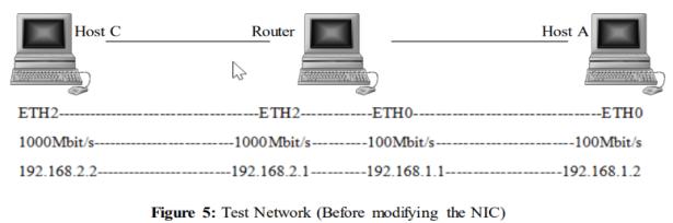
仿真器:tc  (制造丢包)
带宽测量:IPERF,
测试时间:30秒
网卡带宽:1000Mbits/s - 主机C,100Mbits/s - 主机A
最大传输单元(MTU),路由器=1500,主机A&C=1400。
在(前面的实验)生成流量的30秒中,IPERF尽可能多地发送数据包,怀疑大量的数据在数据路径中造成溢出,这可能是剧烈下降的一个可能原因。因此,为了简化分析,只生成了少量的流量(25MB),改变测试条件:
仿真器:tc (制造丢包)
带宽测量:IPERF,
数据大小=25 MB (而不是测试时间:30秒)
网卡带宽:1000Mbits/s - 主机C,100Mbits/s - 主机A
MTU:路由器,主机A,C 均为1400
上面收发两端的网卡带宽不一样,改为一样:
仿真器:tc (制造丢包)
带宽测量:IPERF,
数据大小=25 MB
网卡带宽:主机C,主机A = 10 Mbit/s
MTU:路由器,主机A,C 均为1400
修改网络参数测试结果
仿真器:tc (制造丢包)
带宽测量:IPERF,
数据大小=25 MB
网卡带宽:主机C,主机A = 10 Mbit/s
MTU:路由器,主机A,C 均为1400
单独开启某个参数:
开启 tcp_window_scaling
开启 tcp_adv_win_scale
开启 tcp_ecn
开启 tcp_no_metric_save
以上是发包丢包的影响,而ack包丢包对性能几乎没有影响
除了论文提到的内容,TCP丢包对带宽的影响还与RTT有关:
RTT 可以通过ping 得到。


更多结论见论文:
论文:https://publications.lib.chalmers.se/records/fulltext/193786/193786.pdf
https://download.csdn.net/download/bandaoyu/88571088
概要
观察到在低数据包丢失率(1%)下,性能也受到影响,并且随着数据包丢失率的增加,性能急剧下降。
我们发现TCP甚至无法处理1%的数据包丢失。我们会曾预计性能会出现合理的小幅下降,但实际上观察到性能会大幅下降。我们已经调查了这个问题的性质,并测试了不同的TCP
Linux下的拥塞避免算法(例如Reno、Cubic和H-TCP)。我们也有研究了改变一些TCP参数设置(如TCP_adv_win_scale)的影响,tcp_ecn、tcp_window_scaling、tcp_no_metrics_save。
本文中,对三种不同的拥塞控制算法(Cubic、Reno和H_TCP)进行了比较,并通过多项实验测试对Reno进行了更深入的分析.
测试链接数据丢失和ACK丢失.
首先使用不同的TCP拥塞控制算法,观察它们对带宽率的影响。
然后,更改TCP变量,如高级窗口缩放、ECN值、窗口缩放、TCP no-metric-save值,检查它们在数据包丢失中对保持带宽的作用。
除了实验结果,还包括了一些可能的原因,这些原因是导致观察到的性能率急剧下降的背后原因。此外,实验结果表明,在链接经历数据包丢失时,拥塞控制算法H-TCP的性能优于Cubic和Reno。然而,ACK的丢失并没有太大影响,高达50%的ACK丢失几乎可以容忍,而不会导致性能降低。
关键词:TCP拥塞控制算法,TCP变量,数据丢失,ACK丢失,数据包丢失,带宽率等。
Keywords: TCP congestion control algorithms, TCP variables, Data loss, ACK loss, Packet
loss, Bandwidth rate etc
第1章:大纲
首先,第2章解释了TCP的检测问题表现和相关工作。
在第3章中包含了TCP的各种概念已经简要地描述了拥塞避免算法和TCP变量。
第4章继续描述本文工作中使用的测量工具网络以及分组丢弃的测试场景和测量已经提出。
第五章包含对所执行的所有实验的分析。
第六章对全文进行了总结,
第7章包含结论,
最后第8章讨论了未来的工作。
第2章:问题描述
2.1检测到TCP性能存在问题
2.1 Detected problem in TCP performance
本论文是上一篇论文“SSH Over UDP”的延伸:“在‘基于UDP的SSH’中,为OpenSSH实现了一个基于UDP的解决方案。OpenSSH使用在另一个TCP连接中的TCP连接的隧道来实现其VPN功能。但各种来源声称,在实践中在TCP中使用这种TCP会在两个TCP实现之间产生一些冲突,尤其是在遇到数据包丢失时。因此,一般建议避免TCP中的建TCP隧道(to avoid tunneling TCP in TCP)。他们工作的目标是看看当链路出现数据包丢失时,基于UDP的解决方案是否比基于TCP的解决方案更好。”[4]
隧道是在两个网络之间传输数据的一种安全可靠的方式。隧道协议可以使用数据加密来在公共网络上传输数据。关于隧道、OpenSSH和VPN的详细信息不包括在本文中。
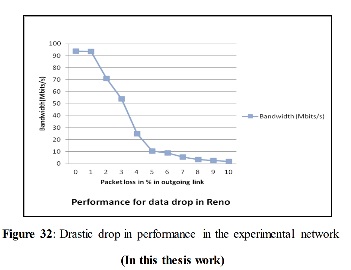
当他们测试不同丢包率的吞吐量时,发现了一个问题。当数据包丢失增加时,吞吐量的下降幅度比预期的要大。找出性能意外下降的原因;因此成为我们研究项目的范围。
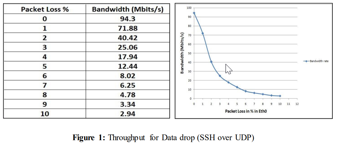
确定的问题如下图1所示。
不丢包时,吞吐量为94.3Mbits/s。只有3%的数据包丢失,吞吐量大幅下降至25.06 Mbits/s,在1%的数据包丢失中,性能从94.3 Mbits/s下降到71.88 Mbits/s,这对用户来说也是容易察觉的.
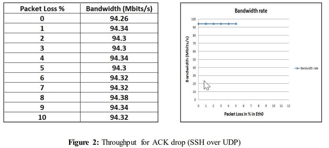
另一方面,从图2中可以看出,当ACK被丢弃时,吞吐量几乎没有变化。
TCP在数据丢弃和ACK丢弃方面表现出不同的行为,这种不同行为背后的原因将在本文稍后讨论。
2.2 相关工作
2.2 Related work 相关工作
Robert Morris [13] has described in the paper, the effect of congestion window size on TCP flow control. The author has identified that TCP‟s minimum congestion window of one packet is the reason behind the reduced ata flow which occurs due to packet loss. Packet transmission rate decreases up to 50% after a single packet loss in the network which in turns generates delays which will be noticeable to the users. Routers also drops packet when their queue is overflowed. TCP is able to overcome the loss of a packet in a single round trip time by increasing its window size larger than 4 packets. The author has suggested a solution by increasing router buffer space together with limits on per-flow queue length. In this paper no external packet loss has been introduced; but for a single packet loss up to 50% decrease in performance has been observed. Hence, initiating external packet loss will end up with huge performance loss.
罗伯特·莫里斯(Robert Morris [13])在论文[13]中描述了拥塞窗口大小对TCP流量控制的影响。作者指出,TCP最小拥塞窗口为一个数据包,这是由于数据包丢失而导致数据流减少的原因.网络中单个数据包丢失后,数据包传输速率会减少多达50%,这反过来会产生用户能够感觉到的延迟。路由器在其队列溢出时也会丢弃数据包。TCP能够通过将其窗口大小增加到4个以上的数据包来克服单次往返时间中数据包的丢失。作者提出了一种解决方案,即增加路由器缓冲区空间,并对每个流的队列长度设置限制。在这篇论文中,没有引入外部数据包丢失;但是单个数据包丢失后,观察到性能最多减少了50%。因此,引起外部数据包丢失将会造成巨大的性能损失。
克里斯蒂安等人[14]提供了TCP的12种不同变体之间的完整比较,即TCP (TCP Reno)及其改进版本(TCP Vegas)、无线网络变体(TCP Veno和TCP Westwood)、高速网络变体(TCP BIC、TCP CUBIC)、卫星网络变体(HSTCP、TCP Hybla、TCP Illinois、Scalable TCP和TCP YeAH),以及一个低优先级版本的TCP (TCP-LP),比较的方面包括实现的吞吐量和公平性。在实现的吞吐量方面,TCP YeAH相较于Scalable TCP和TCP Illinois表现略好。另一方面,在比较公平性与其他TCP变体时;TCP-LP显示出较低的吞吐量。从这篇论文中,我们选取了Reno和Cubic的吞吐量图表,并与我们实验中生成的图表相比较。
本田和Osamu[2]在他们的论文中提出,端到端TCP性能被认为受到链路带宽、传播延迟、MTU和路由器缓冲区大小等因素的影响。作者集中讨论了这些变量以及TCP隧道化如何影响端到端性能。观察结果发现,当网络传播延迟很大时,TCP隧道会导致端到端goodput的下降。缓冲区大小会影响goodput,无论是用于端主机还是隧道连接,这意味着可以通过使用小缓冲区大小来分析goodput的减少。论文还提出,SACK选项可以作为提高goodput的一个替代方法。
Titz[3]指出,在使用TCP隧道时,由于不同TCP栈中有不同的计时器,TCP over TCP被认为是一个不合适的组合,这会导致熔断(meltdown)问题。由于TCP上层存在更快的计时器,它与下层计时器相比进行了更多次的重传,这意味着TCP消息的堆叠使得连接断裂,而不是像普通TCP那样能承受更多的数据包丢失,因为它可以避免拥塞。由于这些问题,作者建议使用UDP作为SSH隧道的TCP替代品。
Canberk、Berk和Jaya Dhanesh[5]关注了TCP熔断问题。假设是使用相同的TCP实现进行隧道连接和转发连接会导致TCP熔断。此外,在一个TCP实现上使用与其它的TCP实现相同的TCP实现,相比单个TCP连接,性能损失几乎增加了一倍。为了避免这种情况,作者建议使用混合的TCP实现,例如对转发连接使用TAHOE实现的TCP,而对另一个连接使用Reno实现的TCP。另一个建议是在隧道传输中使用UDP代替TCP。作者最后得出结论,TCP over TCP并不像人们认为的那么糟糕;此外,使用UDP会产生新的防火墙问题。
Lee等人[6]在他们的论文中提出了TCP和UDP流量的比较,以识别在链路出现瓶颈时哪一种在TCP隧道中表现最好。仅研究了路径MTU大小来分析TCP流的性能,其他因素如链路带宽、缓冲区大小、传播延迟等均未考虑。此外,也没有考虑其他内容,如TCP流的数量、TCP模式和TCP隧道、TCP流的流量模式、TCP拥塞避免算法、SACK选项的存在以及套接字缓冲区的大小。
第3章:TCP概念
在本章中,我们简要介绍了各种TCP拥塞避免算法,本文稍后对不同的TCP变量进行了分析。
3.1 TCP拥塞避免算法
3.1 TCP congestion avoidance algorithms
TCP拥塞避免算法是互联网中拥塞控制的基础[7]。该算法通过观察重传计时器到期和接收到重复ACK来检测拥塞。作为对这种情况的补救措施,发送方将其传输窗口减少到当前窗口大小(即其在途中未被确认的数据包数量)的一半。
有多种类型的拥塞避免算法。例如:Tahoe、Reno、New Reno、Vegas、BIC、CUBIC、H-TCP等。在这项工作中,选择了三种算法进行分析:CUBIC、Reno和H-TCP。当我们安装Linux操作系统时,默认的TCP拥塞避免算法是Cubic。Cubic实现了一种称为二进制拥塞控制(Binary Congestion Control,简称BIC)的增强型拥塞控制算法。BIC拥塞窗口控制功能提高了RTT(往返时间)的公平性和对TCP的友好性。BIC增长函数对于具有短RTT的低速网络中的TCP起到了积极作用。Cubic与短和长RTT都兼容,这意味着良好的可伸缩性。“Cubic的拥塞时间期(两次连续丢包事件之间的时间段)仅由数据包丢失率决定。”Cubic的主要特点是其窗口增长函数是实时定义的,这样它的增长将独立于RTT[8]。
在TCP中,通常对于每个接收到的ACK,拥塞窗口会在每个往返时间(RTT)增加一个段,这种机制称为慢启动。另一方面,当发生数据包丢失时;TCP应用了一种称为乘性减小拥塞避免(MDCA)的机制,将拥塞窗口每个往返时间减少到一半[24]。当发送方在给定时间内没有收到ACK时,就会发生超时。这将触发丢失的数据段的重传。
幸运的是,Reno具有快速重传特征,这减少了发送方在重新传输前的等待时间。但是MDCA机制在Reno中不能正常工作;所以快速重传的数据包也开始在接收端丢失。
因为重传率与接收者的接收能力不成比例,导致大量数据包丢失。因此,Reno仅在非常小的数据包丢失情况下才能表现良好[8,24]。重传率与接收者的接收能力不成比例,导致大量数据包丢失。
H-TCP是我们实验中使用的第三种拥塞避免算法。H-TCP具有一些强大的特性;它可以在高速网络中运作,并且在长距离网络中也表现更好。该协议能够迅速适应现有带宽的变化,使其成为一种带宽高效的协议[15]。
3.2 TCP变量
3.2 TCP variables
在本项工作中,我们假设多个TCP变量会对性能产生影响。由于TCP变量控制的不同特性,我们认为它们应该对性能有一定的影响。为了验证它,本文分析了这四个TCP变量。
tcp_window_scaling启用了一个TCP选项,该选项允许将TCP窗口扩展到一个规模,以适应“大容量胖管道(LPF)”,即具有高带宽时延乘积的链路。在通过大管道传输TCP数据包时,TCP可能会经历带宽损失;因为在等待之前传输的数据段的ACK时,通道并没有被完全填满。TCP窗口扩展选项允许TCP协议对窗口使用一个缩放因子,即使用比原始TCP标准定义的更大的窗口大小,并确保利用几乎全部可用带宽。tcp_window_scaling的默认设置为1,或者说是true。要关闭它,将其设置为0[9,16]。我们分析了这个特性,以减少在通过网络传输大量数据(例如10MB、25MB等)时的性能损失。
tcp_adv_win_scale 可用于套接字的总缓冲空间在输入数据缓冲区(TCP接收窗口)和应用数据缓冲区之间共享。tcp_adv_win_scale用于通知内核应为应用缓冲区保留多少套接字缓冲区大小,以及应为TCP窗口大小使用多少。tcp_adv_win_scale的默认设置为2,这意味着应用缓冲区正在使用总空间的四分之一[9,16]。在我们的实验中,最初它被设置为0,这意味着所有可用内存都分配给了输入数据缓冲区。之后,我们通过将其设置为默认值来检查它对性能的影响。我们使用这个变量的期望是,它将减少的性能损失超过tcp_window_scaling所做的。
tcp_ecn(显式拥塞通知)变量通过在TCP连接中打开显式拥塞通知,当某个路由向特定主机或网络存在拥塞时自动通知主机。tcp_ecn默认是打开的,并且设置为2,另一方面,要关闭它,将值改为0。要在内核中打开它,应将其设置为1[9,16]。选择这个TCP变量是为了检查网络中是否有任何拥塞。
tcp_no_metrics_save控制一个当被打开时允许系统记住上次慢启动阈值(ssthresh)的功能。这个特性修改了第二次测试的结果,并导致错误。当先前连接持有更好结果时,第二次测试的结果将显示一个修改后的结果(更好),而不是原始结果。
tcp_no_metrics_save的默认设置为0,要关闭这个功能,将其设置为1 [9,16]。
选择这个变量的原因是为了观察它对性能的影响,因为它通常提供了整体性能的改善,因为通过记住上次链接的特征,它在搜索拥塞点时不必那么慢地开始。
第4章:测试TCP性能
Chapter 4: Testing TCP performance
本章包含测试网络的描述,包括网络配置以及从测试中获得的数据。给出了我们的初始数据,并与“SSH Over UDP”项目获得的测试数据进行了比较。
4.1测量工具说明
4.1 Description of measurement tools
略
4.2建立网络
4.2 Setting up the network
两台主机(服务器和客户端)以及一台中间计算机(路由器)。中间计算机用来通过引入数据包丢失来干扰服务器和客户端之间的通信。使用Wireshark来分析通过服务器和客户端之间传输的流量。使用Linux网络流量控制工具tc在路由器上引入数据包丢失。然后我们在客户端主机上使用IPERF生成流量,指定了链路上发送的数据量。最大传输单元(MTU)也被设置为其默认值,用于指定允许通过链路转发的最大数据单元。以太网在链路层允许最大1500字节的数据包。在这篇论文工作中,MTU大小被设置为1400字节[18]。
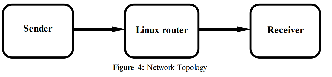
在两个终端主机之间建立了TCP连接。网络接口卡(NIC)在主机A上配置为100Mbit/s,在主机C上配置为1000Mbit/s。后来,它被修改为适用于所有主机。
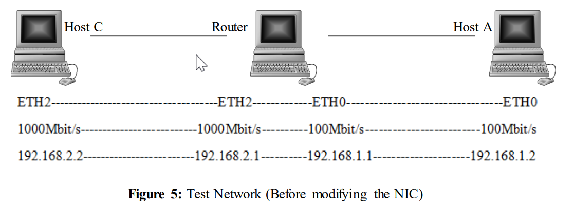
上图是网络的物理图片。为了更清楚地理解测试场景,下面显示了一张更简化的图片。
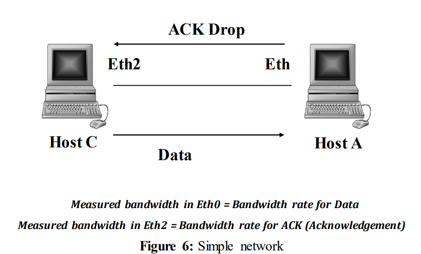
4.3测量TCP丢包的影响
4.3 Measuring the impact of TCP drops
起初,在三台计算机中运行的Linux TCP实现的默认拥塞避免算法称为Cubic(见第3.1章)。TCP变量被设置为它们的默认值(见第3.2章)。使用IPERF,在30秒内测量了性能。
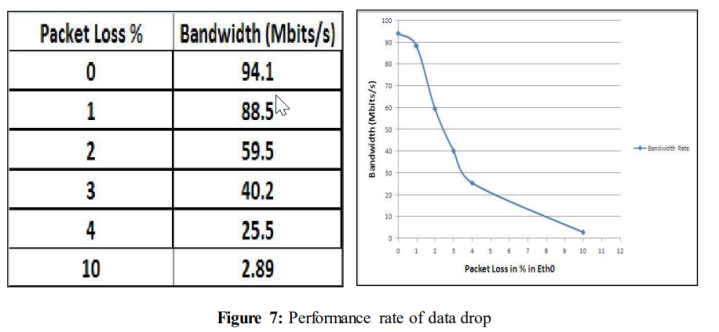
当数据包丢失增加时,性能下降。对于0%的数据包丢失,性能为94.1 Mbits/s,而对于10%的数据包丢失,性能下降到2.89 Mbits/s。初始数据和数据下降的图表在以下小节中展示。
以下实验的测量规格为:
仿真器:tc,
带宽测量:IPERF,
测试时间:30秒
链路带宽:1000Mbits/s - 主机C,100Mbits/s - 主机A
最大传输单元(MTU),路由器=1500,主机A&C=1400。
4.3.1数据链路发生数据丢失时的实验
在第一个实验中,只取了六个测量值来观察当链路经历数据丢失时,网络是否真的经历了急剧下降。在这个实验之后,我们的实验结果证实了“SSH Over UDP”项目[4]获得的结果。
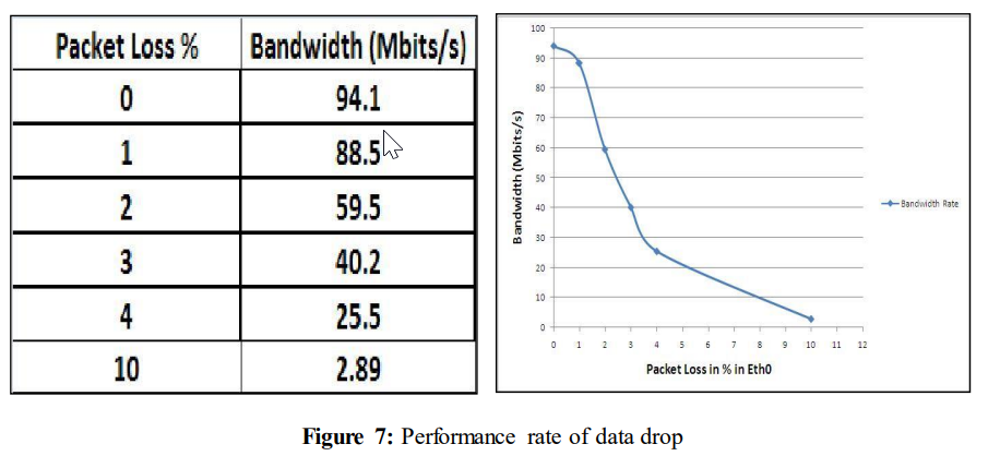
从上图(图7)中可以清楚地看到,当网络中引入数据丢失时,性能急剧下降。当网络中没有数据丢失(或0%的数据包丢失)时,带宽几乎完全用于数据传输。
令人惊讶的是,即使仅引入1%的数据包丢失,性能也会下降到88.5 Mbits/s。当数据丢失达到10%时,性能继续下降到2.89 Mbits/s。
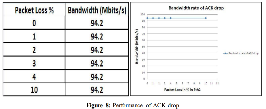
4.3.2 当数据链路经历ACK丢失时的实验
操作六个测量值被记录下来,用来观察在丢弃ACK而不是数据时的性能。没有发现像之前测试(4.3.1)中的性能下降。
在“SSH Over UDP” [4]中提到了当经历数据丢失时发生的剧烈下降情况,在这个网络中也有类似的情况发生。为了验证这种性能的剧烈下降,进行了更多的测量。这些结果在4.3.3、4.3.4、4.3.5和4.3.6中展示。这些实验进行了一些改变。数据不再传输30秒,而是传输25M字节的数据。主机A、C和路由器的MTU设置为1400。
4.3.3 测试CUBIC在数据丢包的情况
4.3.3 Tests with CUBIC when experiencing Data Drop
在进行这个实验时,进行了一些改变。再次选择了CUBIC算法,因为它是运行在两台主机和路由器上的系统的默认拥塞避免算法。下面只列出了与之前实验不同的值。
初始化值:
数据大小=25 MB,而不是测试时间:30秒
MTU=1400,适用于所有主机
使用以上配置进行了两个测试。一个是数据丢失的测试,另一个是ACK丢失的测试。
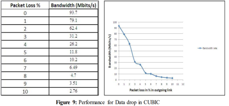
在(前面的实验)生成流量的30秒,IPERF尽可能多地发送数据包。在路由器上使用WireShark来检查网络上的所有这些数据包。对如此大量的流量进行处理和分析对Wireshark来说有些困难,可能是因为Wireshark安装在处理速度较慢(路由器的速度)的CPU上。结果是,Wireshark在每次实验中捕获数据包的时间更长。怀疑大量的数据在数据路径中造成溢出,这可能是剧烈下降的一个可能原因。因此,为了简化分析,只生成了少量的流量(25MB)。
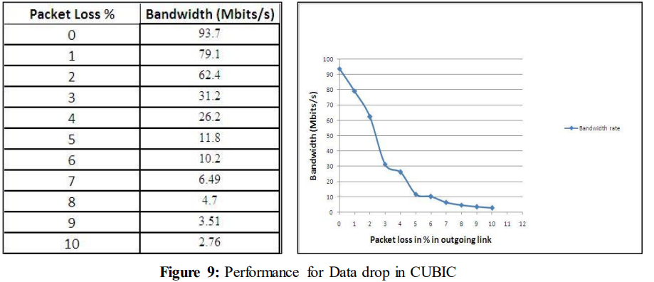
链路发生数据丢失时的体验性能如图9所示。在这里,性能再次随着数据丢失的增加而急剧下降。
4.3.4 测试CUBIC遇到ACK 丢包的情况
4.3.4 Tests with CUBIC when experiencing ACK drop
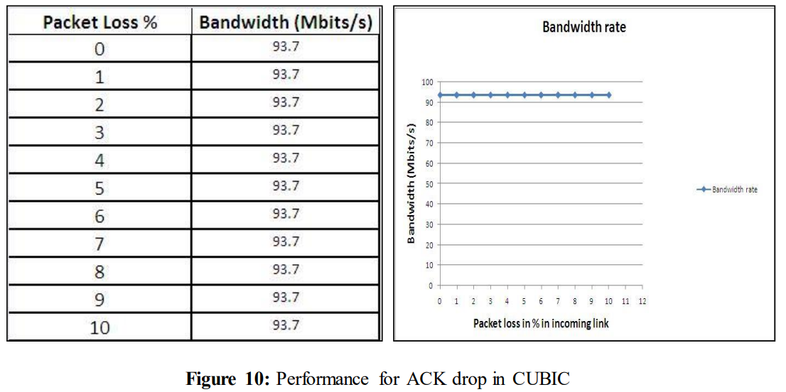
在CUBIC中对ACK丢弃进行了类似类型的实验。得到的结果是
如下图所示
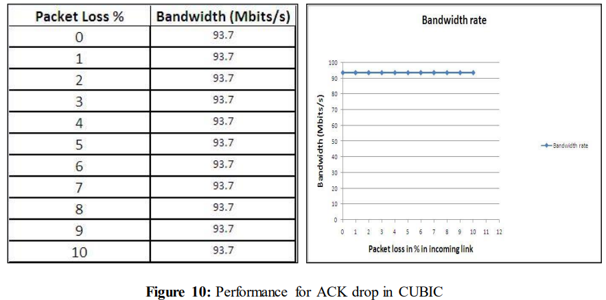
如图10所示,即使在经历10%的ACK丢失时,性能仍保持在93.7 Mbits/s不变。
4.3.5 测试Reno 遇到丢包的情况
4.3.5 Tests with Reno when experiencing Data drop
Similar experiments like 4.3.3 and 4.3.4 was now made with the Reno congestion avoidance algorithm (detailed information about Reno is given in chapter 3 section 3.1). The only change that was made here is the change of congestion avoidance algorithm. Data size was also kept to 25MB. Two tests were made with Reno and performance was measured both for data drop and for ACK drop. The tests outcomes are described below.
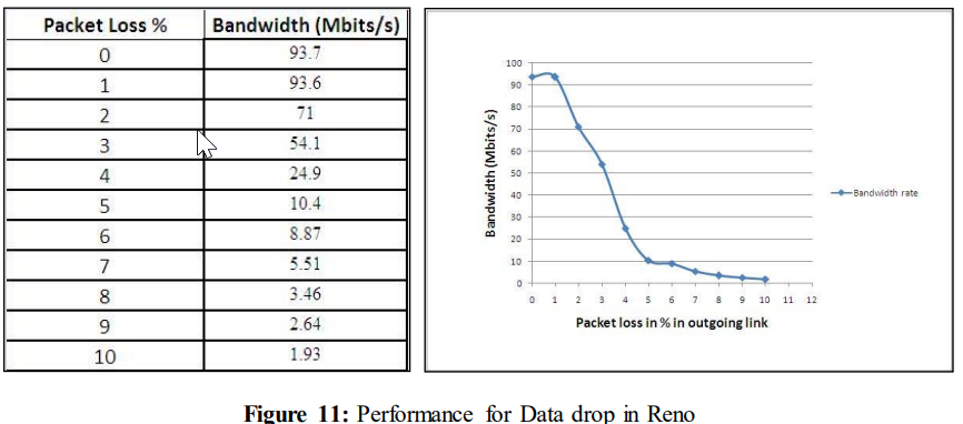
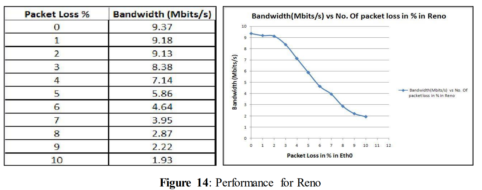
From this analysis it was found that performance becomes more drastic than for CUBIC. The performance was the same when no data loss was introduced but for 10% data loss the rate falls into 1.93 Mbits/s. This rate is lower than the achieved performance in CUBIC (See Figure 8).
4.3.6 测试Reno 遇到 ACK 丢包的情况
4.3.6 Tests with Reno when experiencing ACK drop
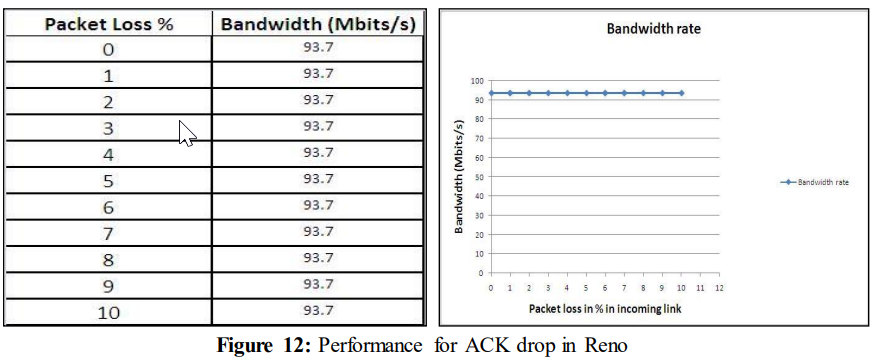
The above figure shows that the ACK drop in the network does not vary when the TCP congestion avoidance algorithm was changed to Reno. The performance remains same even for 10% packet loss 93.7 Mbits/s.
第5章:使用更多算法和TCP变量进行测试
不同的TCP拥塞避免算法在遇到数据丢失时表现出了一些影响,而在ACK丢失时性能并没有改变。
因此,为了观察TCP在数据丢失时的性能,我们测试了不同的拥塞避免算法,如Cubic、Reno和H-TCP,同时改变了四个不同的TCP变量。在开始实验之前,我们配置并更改了一些网络设置。在之前的实验中,三台计算机的NIC(网络接口卡)速度不同,但它们都被设置为NIC支持的最大值。为了减少实验结果可能产生的影响,我们现在使用相同的值对所有NIC进行设置。
5.1 使用不同的拥塞避免算法进行数据丢失实验
在开始之前,将所有NIC的速度设置为10Mbit/s。链接速度被降低(从服务器端的100 Mbit/s降低到10 Mbit/s,从客户端端的1000 Mbit/s降低到10 Mbit/s),以确保网络中具有相同的链接速度。然后在所有三台主机上设置相同的拥塞避免算法。首先,将主机配置为使用Cubic算法,然后更改为Reno算法,最后改为H-TCP算法以观察结果。首先关闭了论文中考虑的所有四个TCP变量(在第3章中有描述)。
以下是实验中的所有重要设置。
用于分析数据的工具:IPERF
所有链接(出站和入站)的链接速度= 10 Mbit/s
数据大小= 25MB
所有三个主机的最大传输单元(MTU)= 1400
5.1.1 CUBIC
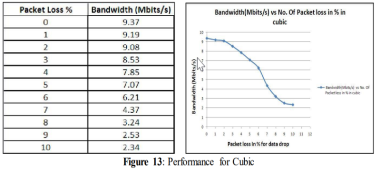
Cubic is the default congestion avoidance algorithm in the Linux operating system. So the first experiment was done with Cubic to observe the performance. From theory (details in chapter 3 sections 3.1) it is already known that Cubic is compatible with both short and long round trip times. It is also supposed to give good performance while links are experiencing data loss.
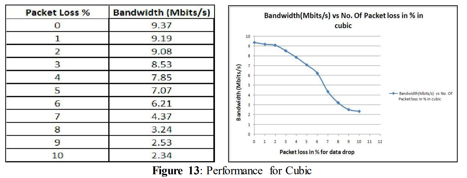
From the above figure (figure 13) it can be seen that when the link was not experiencing any data loss, then the link was fully utilizing its bandwidth and the performance rate was quite high 9.37 Mbits/s. 1% of data loss decreased the performance rate to 9.19 Mbits/s. At 4% data loss, performance went down to 7.85 Mbits/s. After that, the decrease continued and for 10% of data loss performance was down to 2.34 Mbits/s.
5.1.2 RENO
From the earlier theoretical discussion (section 3.1), Reno was not expected to be a competitive congestion avoidance algorithm when experiencing large amount of data loss. Due to its fast retransmission policy, it worked well while small data loss was experienced
5.1.3 H-TCP
According to the theory (chapter 3.1) H-TCP has some strong features to handle data loss over a long distance network. It has also the capability of rapidly adapting changes in existing bandwidth which makes it a bandwidth efficient protocol. Because of these features, H-TCP was one of the selected algorithms among all the congestion avoidance algorithms for this work.
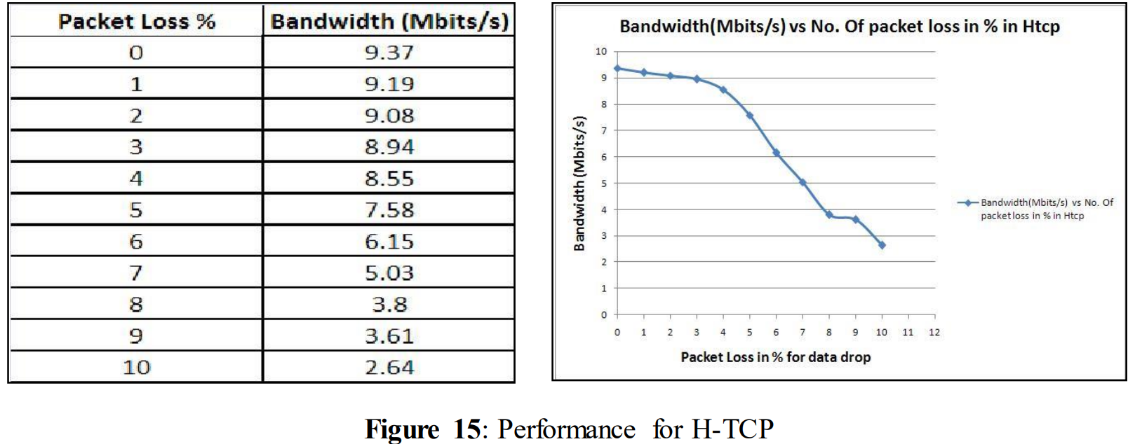
Figure 15 shows the performance of H-TCP. At the beginning when no data loss was introduced to the network, then H-TCP was also utilizing the full bandwidth of the link like Cubic and Reno; and showed a high performance of 9.37 Mbits/s. But later on with an increasing rate of data loss in the network, it also experiences a performance drop. But this drop is slightly better than Cubic and Reno, and from the graph it can be seen that a more drastic drop starts for H-TCP from 5% of data loss. After introducing 10% data loss performance decreases to 2.64 Mbits/s. From these experiments, we can conclude that different congestion avoidance algorithms have impact on performance when links experience data loss. Although the performance of H-TCP was better than Reno and Cubic, for the further experiments with TCP variables Reno was chosen since it had the worst performance among these three congestion avoidance algorithms. It was expected that, if Reno manages to survive with the performance loss; the other two algorithms will definitely show better performance.
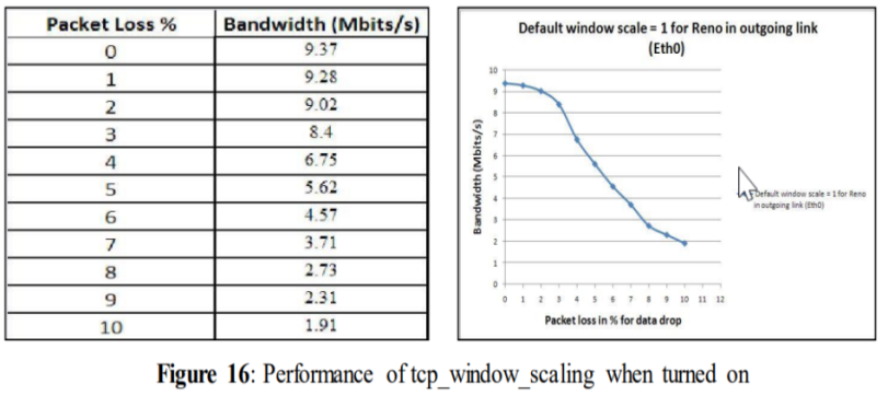
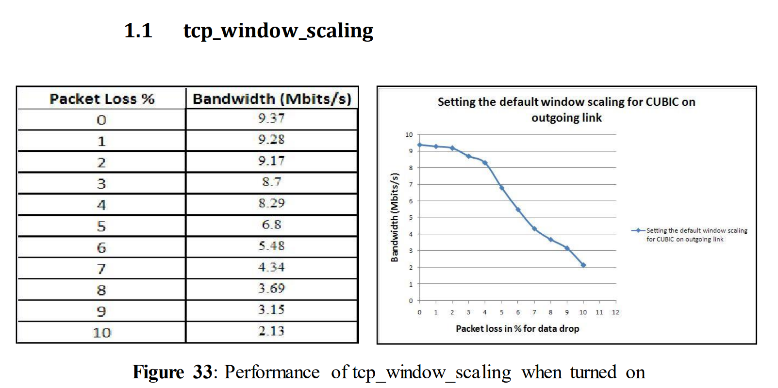
5.1.4使用不同TCP变量进行测试:TCP_window_scaling
5.1.4 Tests with different TCP variables: tcp_window_scaling
A brief description and possible impact of the TCP variables has been described in section 3.2. Initially, tcp_window_scaling was set to 1 or true (which means it was turned on). This means that it will automatically scale the window size according to large fat pipes which ensures utilizing nearly all available bandwidth, which directly reduces the performance loss. Tcp_window_scaling was turned off in the other experiments where the other TCP variables were changed. The network settings for this test are shown below.
Congestion Avoidance Algorithm = RENO
Tools used to analyze the data: IPERF
Link speed, in all links (outgoing and Incoming) = 10 Mbits/s
Data Size = 25MB
MTU for all three hosts = 1400
tcp_window_scaling = 1
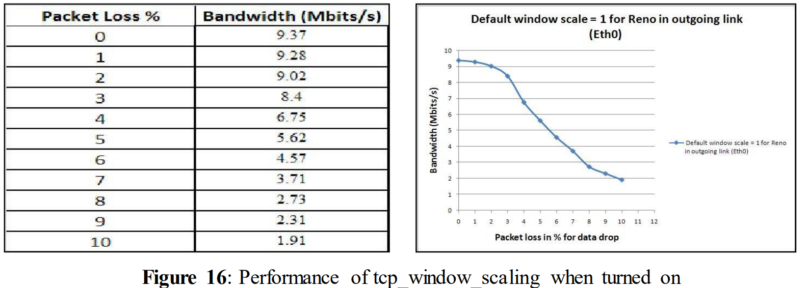
After setting the variable tcp_window_scaling = 1 the above table and graph was obtained. Even now with an increased amount of data loss, performance starts decreasing. For 3% of data loss, performance decreases to 8.4 Mbits/s, and for 10% data drop performance is down to 1.91 Mbits/s. Although this TCP variable has the function to reduce performance loss, in this case it doesn´t show any remarkable changes compared to figure 14 where tcp_window_scaling is turned off.
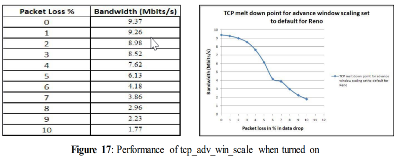
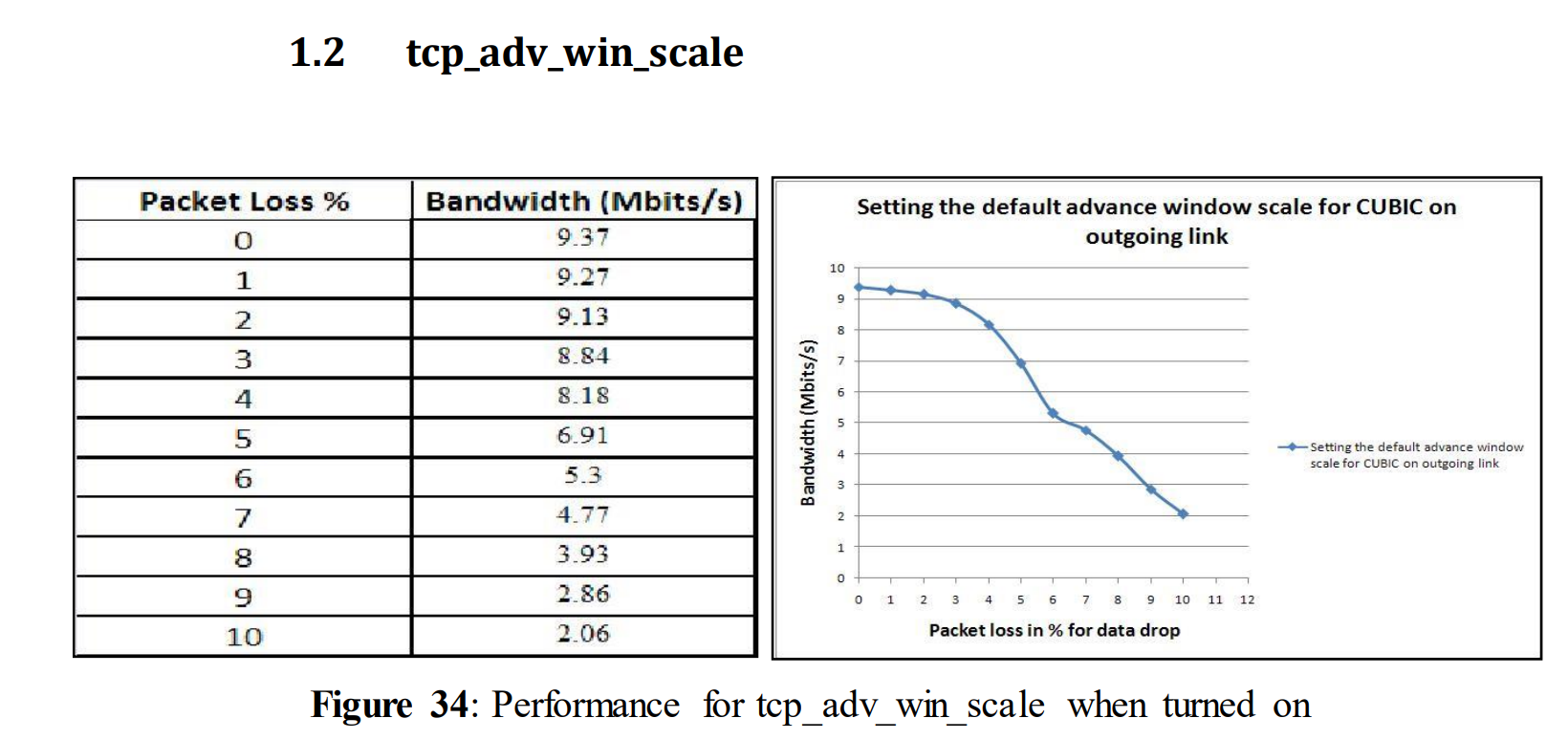
5.1.5使用不同TCP变量的测试:TCP_adv_win_scale
5.1.5 Tests with different TCP variables: tcp_adv_win_scale
In figure 14 tcp_adv_win_scale was turned off. Tcp_adv_win_scale was initially turned on and set to its default value 2, which means that the application buffer was using one fourth of the total space (details given in section 3.2). This TCP variable can be turned off by setting its value to 0. So, to observe the impact on performance of tcp_adv_win_scale, it was turned on and the other TCP variables were turned off. tcp_adv_win_scale= 2
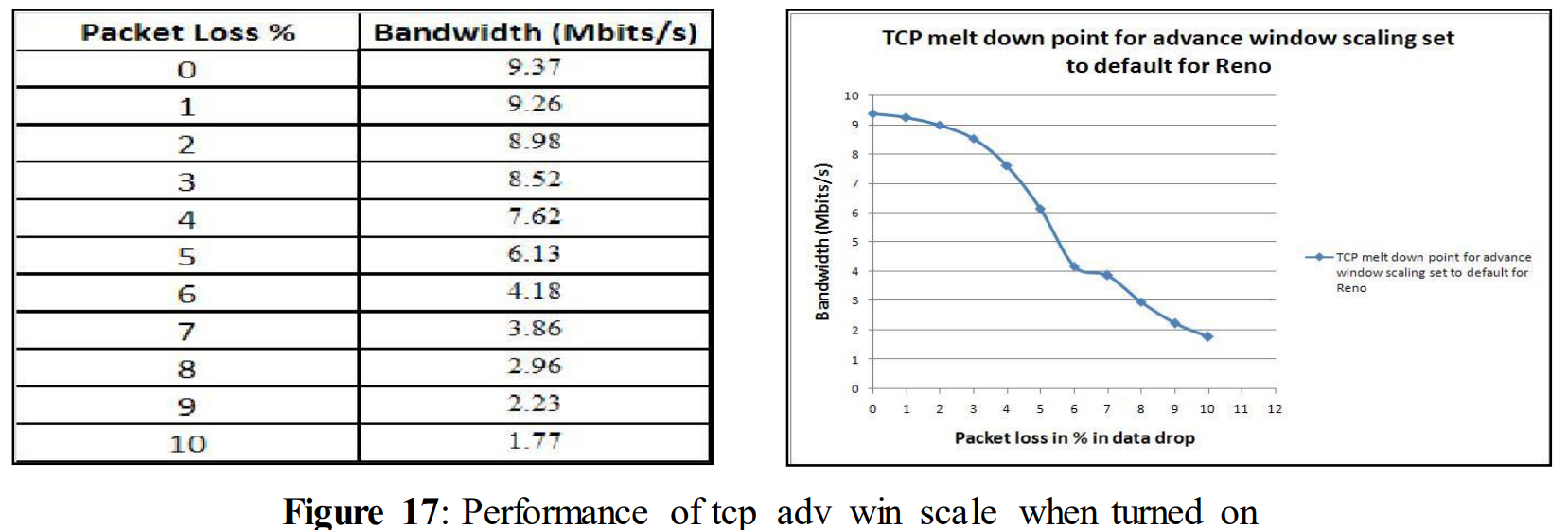
From the above figure, it can be seen that a drastic drop was noticed from 4% of data loss and ended up with only 1.77 Mbits/s for 10% data drop. As in our previous test, it was not able to give a good performance for 10% data drop. However, when compared to figure 14, it performed slightly better from the beginning when packet loss was rather small.
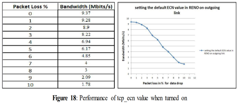
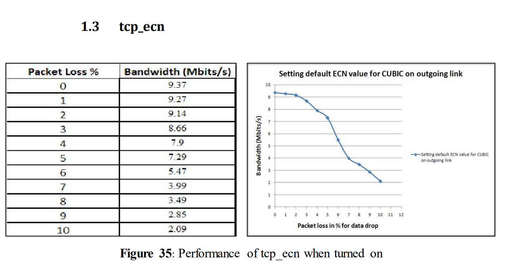
5.1.6使用不同TCP变量的测试:TCP_ecn
5.1.6 Tests with different TCP variables: tcp_ecn
In the earlier test shown in figure 14 tcp_ecn was turned off (tcp_ecn=0). Tcp_ecn (Explicit Congestion Notification) is by default turned on (tcp_ecn=2). In this test, we wanted to observe the impact on performance when tcp_ecn was turned on and compare it with the performance shown in figure 14. This variable was turned on only in this particular experiment. In other cases it was set to 0.
tcp_ecn = 2 (default)
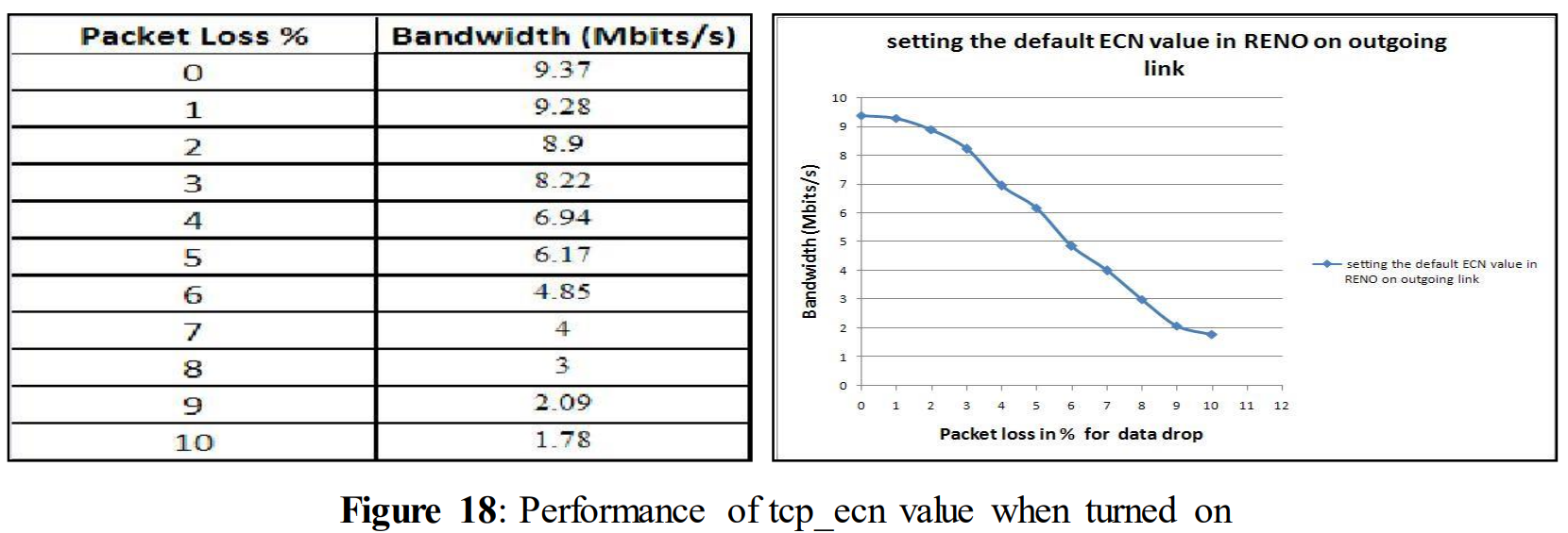
Figure 18 shows the experimental result when tcp_ecn is set to 2. After analyzing the above graph it can be seen that turning on this variable doesn´t make it differs very much from the experimental result of figure 14. As before, performance drops drastically when data drop exceeds 4%.
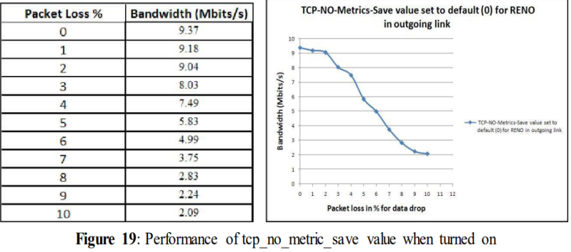
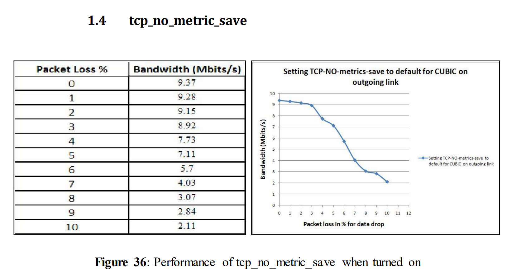
5.1.7不同TCP变量的测试:TCP_no_metrics_save值
5.1.7 Tests with different TCP variables: tcp_no_metrics_save value
The value of tcp_no_metrics_save was set to 1(save functionality disabled) in figure 14. But tcp_no_metrics_save value is by default set to 0(save functionality enabled). It controls a function that has got a function of remembering the last slow start threshold (ssthresh) when it is turned on. So we chose this variable to observe if it affects performance. A performance increase was expected from this experiment because it normally offers an overall performance improvement by remembering the previous results of the link, so it does not have to start slowly while searching for the congestion point. This functionality was turned off in all other experiments except in this experiment.
tcp_no_metriic_save = 0
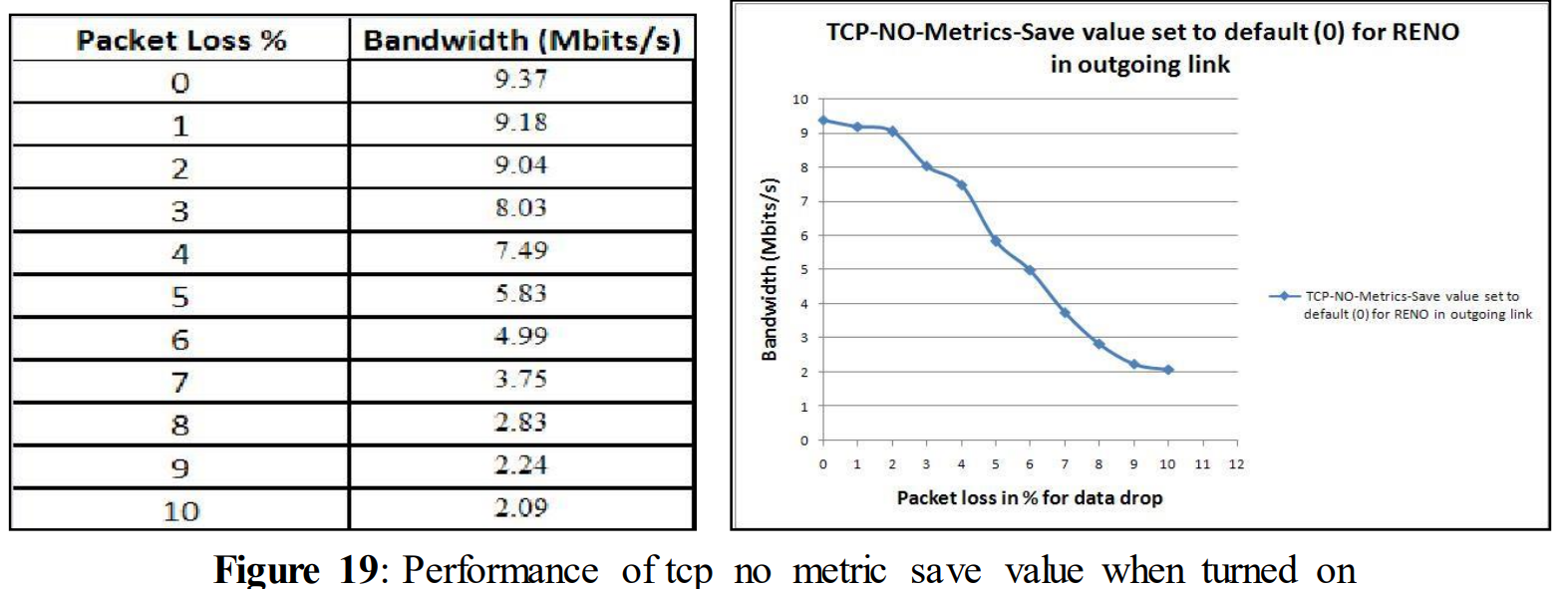
From the above figure (Figure 19) it can be observed that the performance was slightly better compared to Figure 14. For 10% of data drop the performance becomes 2.09 Mbits/s while in figure 14 for 10% data drop the performance was 1.93 Mbits/s.
5.2 针对ACK丢包的不同拥塞避免算法的实验
5.2 Experiments with different congestion avoidance algorithms for ACK loss
5.2.1 CUBIC/RENO/H_TCP
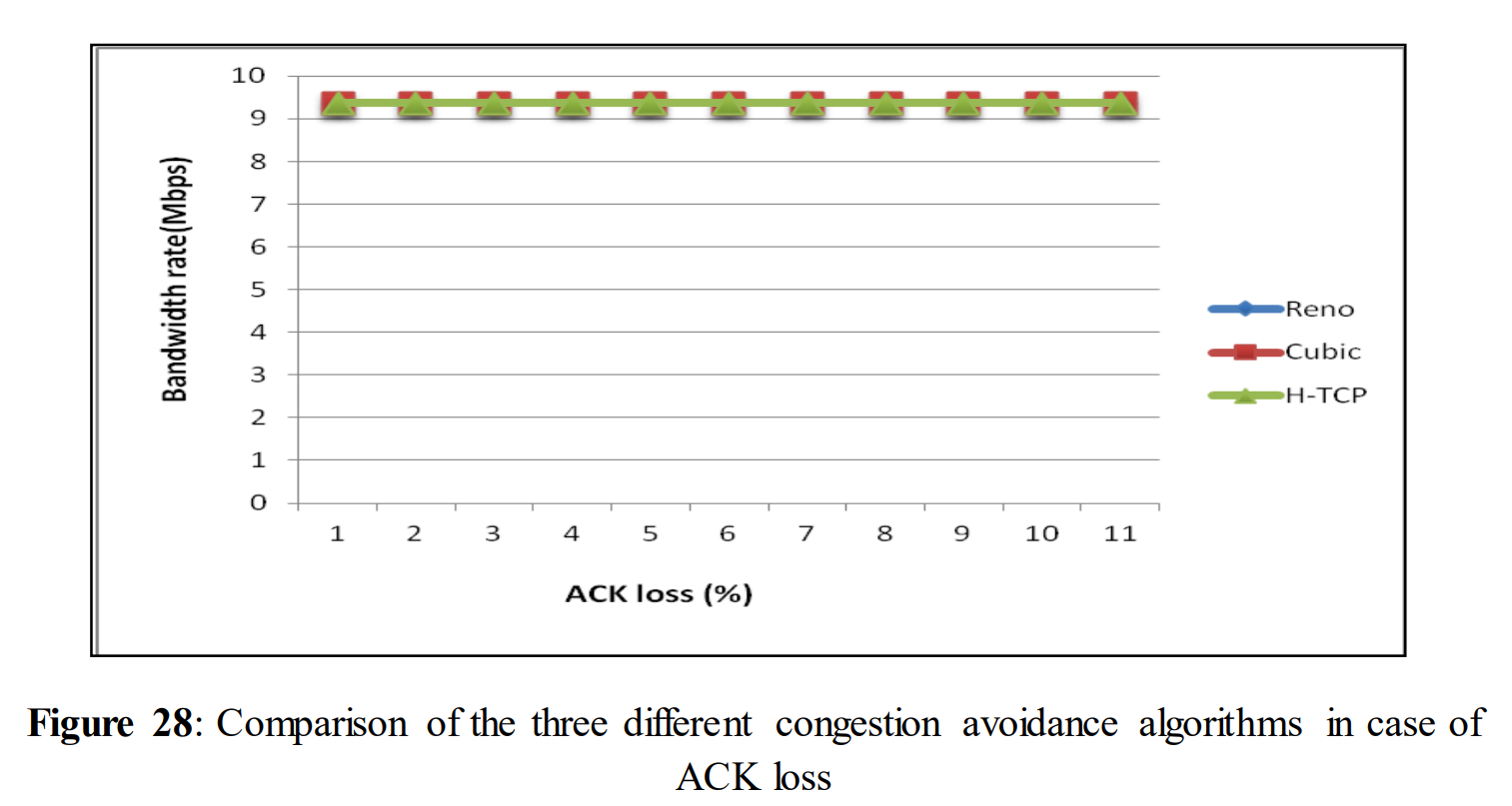
All of three congestion avoidance algorithms have given the same experimental results when Acknowledgements are dropped. All TCP variables are turned off here for this experiment.
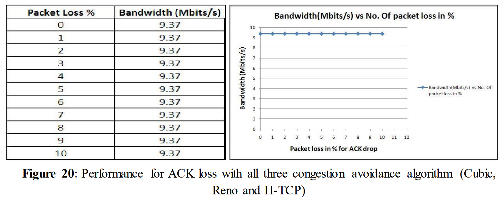
Figure 20 shows the performance while links are experiencing ACK loss. It can be seen that there was no change in performance regardless of whether the loss was 1% or 10% for all three congestion avoidance algorithms. This experiment shows that even a relatively high amount of acknowledgement loss doesn´t have any impact on the performance. But to make this statement stronger further experiments with ACK loss have been done.
From experiment 5.2.1 it has been understood that small amount of ACK loss doesn´t have any impact on the performance. So the ACK loss was increased ten times from the previous test. That means 10%, 20%, 30%…100% of ACK loss was introduced to the network instead of 1%, 2%, 3%...10%.
Now, another test was done with congestion avoidance algorithm Reno; applying the increased amount of ACK loss. The obtained figure is given below.
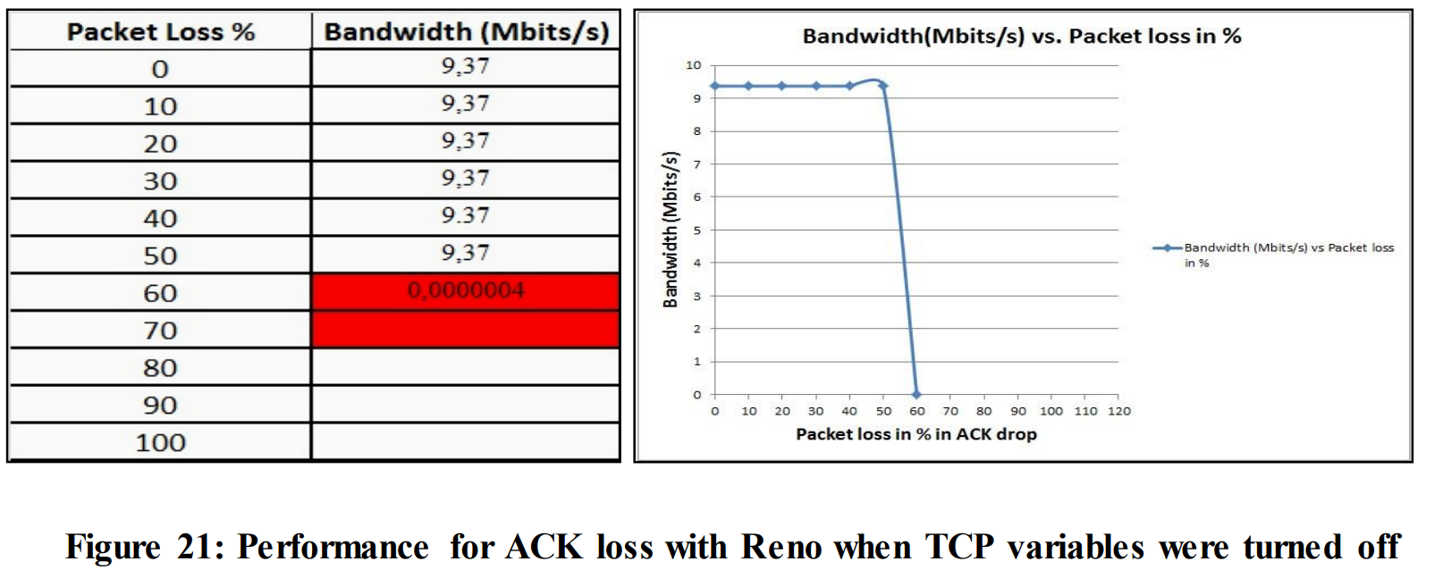
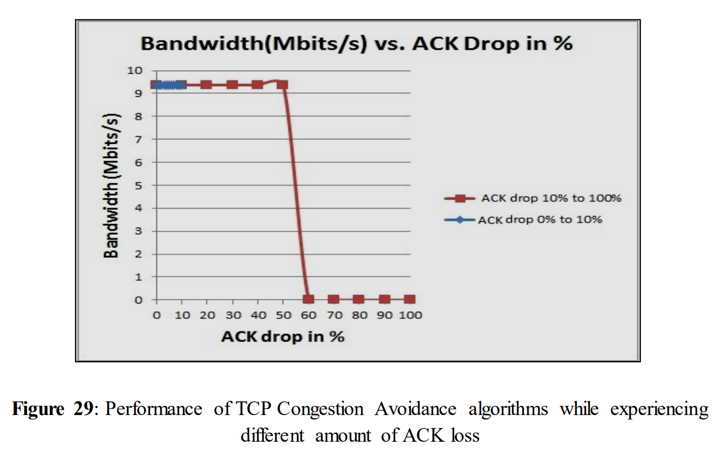
In figure 21, after increasing the loss, performance remains unchanged till 50% of ACK loss. At 60% of ACK loss the performance dropped to almost 0(i.e. 0.0000004). Now, similar tests were done with the four TCP variables by turning them on separately in each test. To compare the performance of four TCP variables (when they were turned on) with figure 21, the following tests (5.2.2, 5.2.3, 5.2.4, 5.2.5) were done.
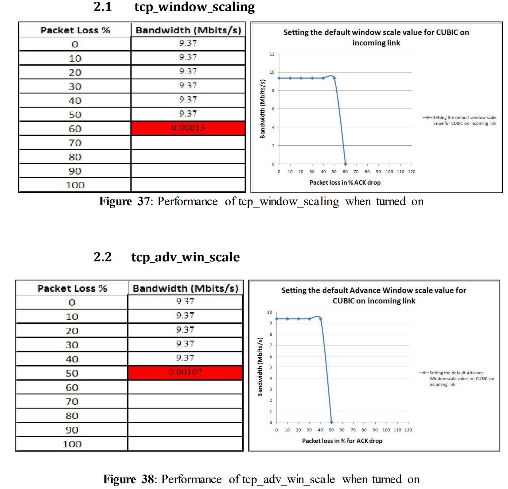
5.2.2使用不同TCP变量的测试:TCP_window_scalin
5.2.2 Tests with different TCP variables: tcp_window_scalin
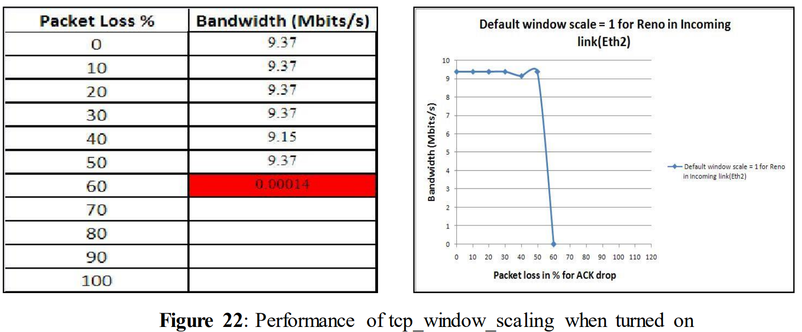
The first test was done with tcp_window_scaling. It was turned on for this experiment
tcp_window_scaling = 1 for ACK loss
5.2.3使用不同TCP变量的测试:TCP_adv_win_scale
5.2.3 Tests with different TCP variables: tcp_adv_win_scale
In this test tcp_adv_win_scale was turned on (set to 2). The meaning of the value has been discussed in 5.15 during the experiments of data loss. The same experiments were done for ACK loss to see its impact on the performance.
tcp_adv_win_scale = 2
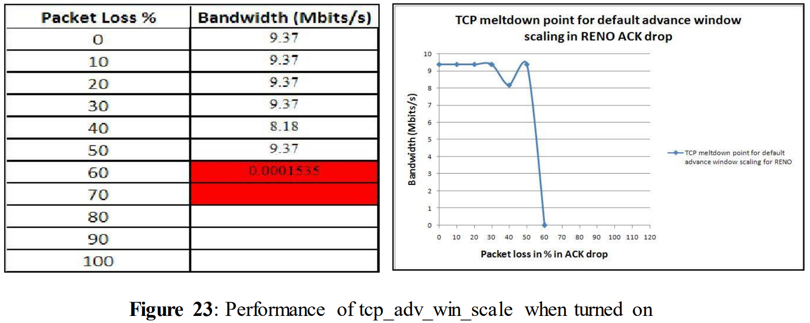
The above figure shows a drop in performance at 40% ACK loss, otherwise there is no significant difference from earlier experiments. As before, when we have reached 60% loss; performance was down to 0 (0.001535).
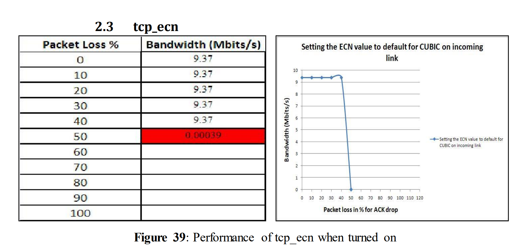
5.2.4使用不同TCP变量的测试:TCP_ecn
5.2.4 Tests with different TCP variables: tcp_ecn
In this test; tcp_ecn (Explicit Congestion Notification) was turned on, so that explicit notifications were delivered while congestion occurred.
tcp_ecn = 2 for ACK loss
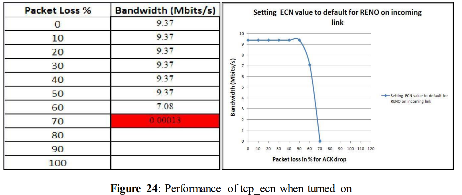
Performance was unchanged up to 50% of ACK loss i.e. 9.37 Mbits/s. For 60% of ACK loss performance dropped to 7.08 Mbits/s. However, compared with the figure 21 tcp_ecn was able to improve the performance at 60% quite significantly, but it wasn‟t able to handle 70% of ACK loss.
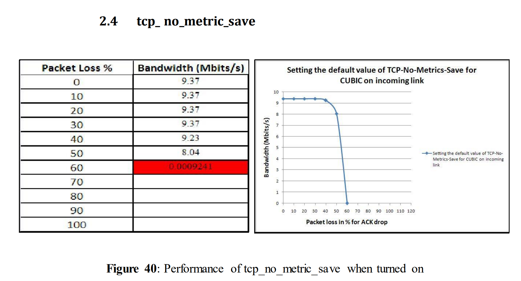
5.2.5使用不同TCP变量的测试:TCP_no_metric_save值
5.2.5 Tests with different TCP variables: tcp_no_metric_save value
Now, tcp_no_metric_save value was turned on to compare its performance with figure 21. The graph for ACK loss is shown in figure below. tcp_no_metric_save = 0 for ACK loss
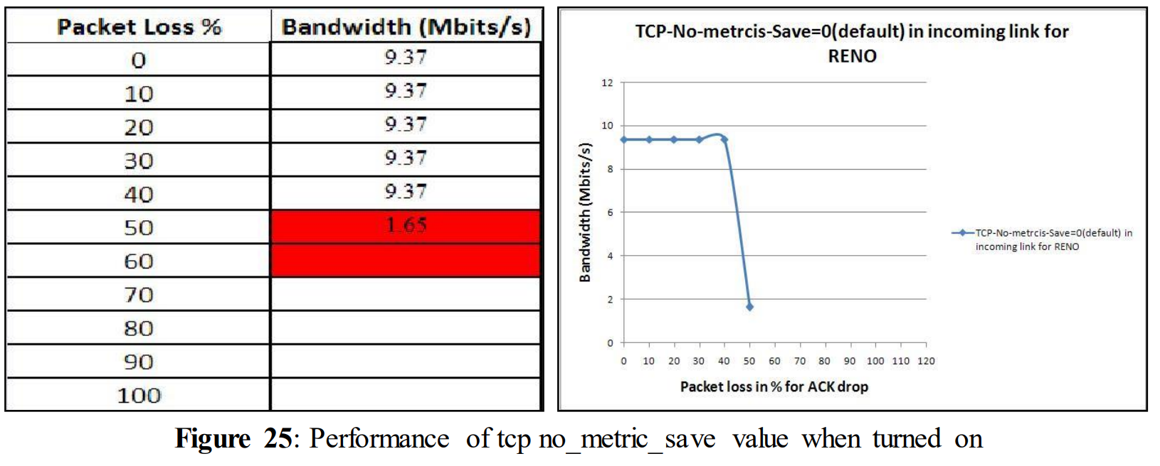
In figure 25 it can be seen that performance drops already at 50% of ACK loss and goes down to 1.65 Mbits/s. To conclude the experiments with ACK loss and as seen in the above graphs (Figure 21 to Figure 25) it is clear that changing the values of TCP variables doesn´t have much impact on performance when experiencing ACK loss. Some extra experiments have been done with TCP variables both for data loss and ACK loss with Cubic in order to verify the results of Reno. But there were no major differences found in the results. These figures are presented in the appendix to avoid redundancy.
第6章:讨论
Chapter 6: Discussion
Chapter 5 contains description of all the experiments that were done during this thesis work. The results from these tests are presented in this chapter.
6.1 数据包丢失时的实验结果
6.1 Outcome from the experiments when link experiencing Data loss
During data drop, the analysis of the three different congestion avoidance algorithms didn‟t show that much dissimilarity in performance drop from each other. A huge drop was observed for all the congestion avoidance algorithms. Only H-TCP showed slightly better performance (figure 26).
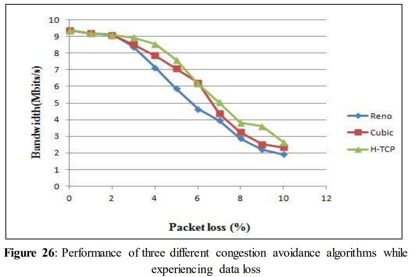
In figure 26 for 1% packet drop the bandwidth rates were 9.18, 9.19, and 9.19 for Reno, Cubic and H-TCP respectively. For 5% data drop these bandwidth decreased to 5.86, 7.07 and 7.58. While introducing 10% data loss the bandwidth rates declined to 1.93, 2.34 and 2.64. Four different TCP variables (tcp_window_scaling, tcp_ecn, tcp_adv_win_scale, tcp_no_metrics_save) were analyzed first with their default values and then by changing them one by one. Performance drop was quite similar for all four variables while they were turned off. A small raise in performance was observed when disabling tcp_no_metrics_save
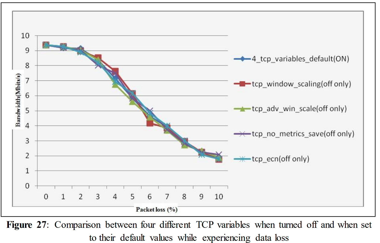
In figure 27 for 1% packet drop the bandwidth rates were 9.18, 9.26, 9.28, 9.18 and 9.28 with the different TCP variables (tcp_window_scaling, tcp_ecn, tcp_adv_win_scale, tcp_no_metrics_save) set to default and turning them off (individually) respectively. For 5% performance drop the bandwidth rates fall down to 5.86, 6.13, 5.62, 5.83 and 6.17. While introducing 10% data loss the bandwidth rates declined to 1.93, 1.77, 1.91, 2.09 and 1.78 respectively.
6.1 ACK数据包丢失时的实验结果
6.2 Outcome from the experiments when link experiencing ACK loss
During the experiments, when the link was experiencing ACK drop, it could be seen that performance was not affected by a small number of acknowledgement drops. In the case of data drops, even for 1% packet drop, a decrease in performance was noticeable. While the ACK drop occurred, performance was unchanged for the link and remained constant at 9.37 Mbits/s even when the link experienced 10% of ACK loss.
 To see the performance when link experiences a high amount of ACK drops, we have increased the quantity of ACK drop to 10 times. Instead of 1%, 2%, 3%... 10% ACK drop rate, we observed the performance for 10%, 20%, 30%.....100% ACK drop. In these experiments; a temporary performance drop was noticed after 40% acknowledgement drop. At one stage congestion occurred in the network when the ACK drop was huge (70%). The same experiments were repeated three times to ensure these results. Each time it showed performance drop after 40% acknowledgement drop and communication completely stalled at 60% acknowledgement drop.
We also tested to use different congestion avoidance algorithms (Reno, H-TCP, and Cubic) and when different TCP variables (tcp_window_scaling, tcp_ecn, tcp_adv_win_scale, tcp_no_metrics_save) were set to their default values. This shows that performance doesn‟t fall with a small amount of ACK drops. Experiments were also done by turning off TCP the variables (tcp_window_scaling, tcp_ecn, tcp_adv_win_scale, tcp_no_metrics_save). This time a huge drop was observed when exceeding 50% of acknowledgement drop.
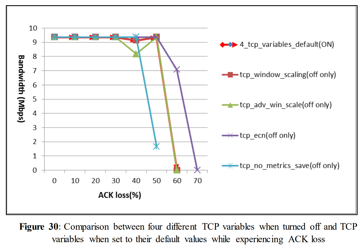
In figure 30 when TCP variables were set to default (ON) bandwidth remain constant at 9.37 Mbps from 0% to 40 % ACK drop. For 50% ACK drop bandwidth declined to 0.0000004 Mbps. While TCP variables were turned off one by one, tcp_window_scaling and tcp_adv_win_scale showed a huge decrease in bandwidth rates with 60% ACK drop, at that time the bandwidth rates were 0.00014 Mbps and 0.0001535 Mbps respectively. With 70% ACK drop for tcp_ecn; bandwidth declined to 0.00013 Mbps. TCP_no_metrics_save showed a very low bandwidth rate which was 1.65 Mbps for 50% ACK drop.
6.3 RENO 丢包时出现数据时急剧下降的可能原因
6.3 Possible reason behind the drastic drop when link experiencing Data loss in RENO
The department of Information Engineering of University of Pisa of Italy has published a paper on the analysis of the TCP‟s behavior where they faced no packet loss [14].
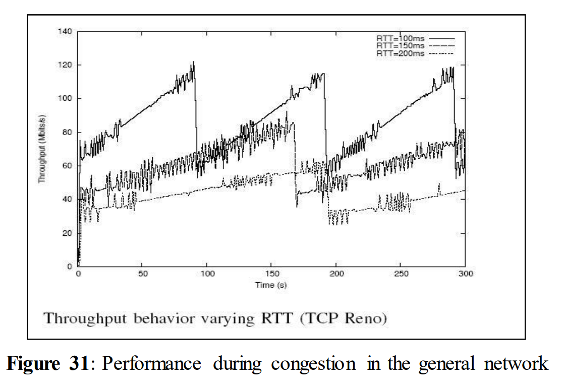
When Reno was running as the congestion control algorithm, even for a single packet loss, the throughput observed by them decreased from 120 to 60 Mbps which means that current transmission rate is temporarily decreased to 50% (Figure 31) and then increases linearly until another loss occurs. The design of the congestion avoidance methods can be likely the reason behind the remarkable performance drop during heavy packet loss. Since transmission rate goes down to 50% for each lost packet and then the transmission rate is increased linearly. But after the next packet loss, transmission rate again decreases to 50% of the last value. There will be an imbalance in increase (linear) and decrease (cut in half) in transmission rate which will decrease the performance too fast. This can be one of the reasons behind declined performance of TCP.
 Our findings are supported by [25] where the authors have simulated TCP Reno behavior during multiple packet loss. In Reno, upon receiving duplicate ACKs, the sender initiates a fast retransmission mechanism. When the fast retransmit mechanism signals congestion, the sender, instead of returning to Slow Start uses a Multiplicative Decrease Congestion Avoidance (MDCA) which is a part of the fast recovery mechanism. During transmission dropping two packets in the same window often leads to force the Reno sender to wait till retransmission timeout. During this drop, if the congestion window is less than 10 packets or the congetion window is within two packets of the receiver‟s advertised window Fast Recovery mechanism will be initiated. When three packets are dropped in the single window of data and the number of packets between the first and second dropped packets is less than 2+3W/4 (W is the congestion window just before the Fast Retransmit) the Reno sender will wait for a retransmit timeout. When four packets are dropped in a single window Reno sender have to wait for a retransmit timeout. With the increased number of dropped packets in the same window, the likelihood to wait till retransmits occurs increases, which disrupts data transmission and halts the transmission at a certain stage. When the fast retransmission mechanism is disrupted, the fast recovery mechanism will not be able to perform properly [25]. In our thesis work, by introducing packet loss we have dropped the packets randomly. So, there is a high possibility that more than one packet has been dropped in the same window. This indicates an inefficient use of the fast retransmission and fast recovery mechanism which can be a probable reason behind huge performance drop
第7章:结论
In order to understand the reason behind TCP‟s drastic drop behavior with increasing packet loss, three different congestion avoidance algorithms (Reno, H-TCP, and Cubic) along with four different types of TCP variables (tcp_window_scaling, tcp_ecn, tcp_adv_win_scale, tcp_no_metrics_save) have been analyzed. The department of Information Engineering of University of Pisa of Italy has mentioned in a paper that they have also observed a decrease in transmission rate with single packet loss which leads to significant performance drop; similar to the drastic performance drop we have observed in our thesis work. In a small network we have analyzed the behaviour of TCP Reno by introducing packet loss. TCP Reno performed well when no packet loss was introduced, but by introducing 1% packet loss, the performance went down from 9.37 Mbps to 9.18 Mbps which means a 2% performance decrement and it linearly decreases. When reaching 10% packet loss, performance went down to 1.93 Mbps. A similar type of experiment was done while introducing external ACK loss. A small amount of ACK loss did not affect performance at all; it remained constant at 9.37 Mbps. But a large amount of ACK loss for example 40% ACK loss caused performance to drop from 9.13 Mbps to 8.18 Mbps and with 60% ACK drop, performance went down to 0.00014 Mbps. Comparing Cubic and Reno, Cubic performed better. In Cubic the performance was constant at 93.7 Mbps till 60% of ACK drop. In Reno, performance decreased to 17.9 Mbps while link was experiencing 30% ACK drop and for 60% ACK loss, performance declined to 0% like Cubic. ACK loss is not as serious as loss of data packets since they are accumulative, meaning that a missing ACK will be covered for when the next ACK is delivered. However, when excessive ACK loss occurs, the sender has to retransmit the packets again, and it is likely that high ACK loss rate will rapidly increase the amount of retransmitted packets that, again will be lost and retransmitted, will create huge load in the network which likely is the reason for this performance drop. We have compared three congestion avoidance algorithms with respect to packet loss; Reno‟s performance was the worst among the three algorithms. In Theory H-TCP was expected to be the best performing algorithm because this algorithm uses network resources efficiently, it is also able to acquire and release bandwidth fast in response to changing network conditions. H-TCP is also suitable for using with simple and complex networks. Our analysis also showed that performance improved slightly with H-TCP. We have also investigated how Four TCP variables (tcp_window_scaling, tcp_ecn, tcp_adv_win_scale, tcp_no_metrics_save) affected performance and they only slightly changed performance. Most of the experiments were done with Reno. Because Reno was the worst performing algorithm; if Reno can survive through the drastic drop in the performance with the increment of packet loss than other two algorithms will likely show better results in the same environment, in our experiments when experiencing packet loss and ACK loss. In the case of packet loss all the four TCP variables show almost the same drastic drop as before. Experiments were done by turning off the TCP variables for both packet drop and ACK drop; slightly better performance was observed (2.09 Mbps) with tcp_no_metric_save. On the other hand, a huge amount of ACK loss for example, 40% ACK loss caused performance to drop to 8.18 Mbps and 60% ACK drop to 0.00014 Mbps. In conclusion we can conclude from all the experimental results that congestion control algorithm H-TCP performs slightly better than Cubic and Reno while the link was experiencing packet loss. A small amount of ACK loss doesn´t affect the performance while a large amount of ACK loss could not be handled by TCP.
附录
1. CUBIC 拥塞算法下不同参数时丢包的测试
Tests with different TCP variables in CUBIC for Data loss
 2. CUBIC 拥塞算法下不同参数时ACK丢包的测试
2 Tests with different TCP variables in CUBIC for ACK loss
论文2:带宽与丢包(Throughput versus loss)
|
| Throughput versus loss Les Cottrell Last Update: February 16, 2000 Central Computer Access | Computer Networking | Internet Monitoring | IEPM | Tutorial on Internet Monitoring |
|

Introduction
The macroscopic behavior of the TCP congestion avoidance algorithm by Mathis, Semke, Mahdavi & Ott in Computer Communication Review, 27(3), July 1997, provides a short and useful formula for the upper bound on the transfer rate:
where:
Rate: is the TCP transfer rate or throughputd
MSS: is the maximum segment size (fixed for each Internet path, typically 1460 bytes)
RTT: is the round trip time (as measured by TCP)
p: is the packet loss rate.
Note that the Mathis formula fails for 0 packet loss. Possible solutions are:
- You assume 0.5 packets were lost. Eg. assume you send 10 packets each 30 mins for 1 year then 48 (30 min intervals in day) * 10 packet *365 days = 175200 pings or a loss rate of 0.5/175200 = 0.00000285.
- You take the Padhye estimate (see bwlow) for 0 packet loss, i.e. Rate = Wmax / RTT. The default Linux Wmax is 12k8Bytes (see Linux Tune Network Stack (Buffers Size) To Increase Networking Performance).
An improved form of the above formula that takes into account the TCP initial retransmit timer and the Maximum TCP window size, and is generally more accurate for larger (> 2%) packet losses, can be found in: Modelling TCP throughput: A simple model and its empirical validation by J. Padhye, V. Firoiu, D. Townsley and J. Kurose, in Proc. SIGCOMM Symp. Communications Architectures and Protocols Aug. 1998, pp. 304-314. The formula is given below (derived from eqn 31 of Padhye et. al.):.
if w(p) < wmax
Rate = MSS * [((1-p)/p) + w(p) + Q{p,w{p}}/(1-p)] /
(RTT * [(w{p}+1)]+(Q{p,w{p}}*G{p}*T0)/(1-p))
otherwise:
Rate = MSS * [((1-p)/p)+ wmax+Q{p,wmax}/(1-p)] /
(RTT * [0.25*wmax+((1-p)/(p*wmax)+2)] + (Q{p,wmax}*G{p}*T0)/(1-p)])
Where:
We have assumed the number of packets acknowledged by a received ACK is 2 (this is b in the Padhye et. al. formula 31)
wmax is the maximum congestion window size
w{p} = (2/3)(1 + sqrt{3*((1-p)/p) + 1} from eqn. 13 of Padhye et. al. substituting b=2
Q{p,w} = min{1,[(1-(1-p)3)*(1+(1-p)3)*(1-(1-p)(w-3))] /
[(1-(1-p)w)]}
G{p} = 1+p+2*p2+4*p3+8*p4+16*p5+32*p6 from eqn 28 of Padhye et. al.
T0 = Initial retransmit timeout (typically this is suggested by RFCs 793 and 1123 to be 3 seconds).
Wmax = Maximum TCP window size (typical default for Solaris 2.6 is 8192 bytes)
If you are tuning your hosts for best performance then also read Enabling High Performance Data Transfers on Hosts and TCP Tuning Guide for Distributed Application on Wide Area Networks. Also The TCP-Friendly Website summarizes some recent work on congestion control for non-TCP based applications in particular for congestion control schemes that maintain the arrival rate to at most some constant over the square root of the packet loss rate.
A problem with both formulae for 0 packet loss is that the throughput depends on RTT which may change by little from year to year for a host pair with terrestrial wired links. Thus the formulae start to fail for long term trends unless one knows the Wmax as a function of time for such pairs of hosts. Unfortunately this is typically only known by the system administrators and may change with time.
Measurement of MSS
On June 7-8, 1999, we measured the MSS between SLAC and about 50 Beacon sites by sending pings with 2000 bytes and sniffing on the wire to see the size of the response packets. Of the 48 Beacon site paths pinged all except 1 responded with an MSS of 1460 bytes (packet size of 1514 bytes as reported by the sniffer), and the remaining 1 (nic.nordu.net) was unreachable.
Validation of the formula
Between May 3 and May 15, 1999, Andy Germain of the Goddard Space Filght Center (GSFC) made measurements of TCP throughput between GSFC and Los Alamos National Laboratory (LANL). The measurements were made with a modified version of ttcp which, every hour, sent data from GSFC to LANL for 30 seconds and then measured the amount of data transmitted. From this a measureed TCP throughput was obtained. At the same time Andy sent 100 pings from GSFC to LANL and measured the loss and RTT. These loss and RTT measurements were plugged into the formula above to provide a predicted throughput. We then plotted the measured TCP throughput (ttcp) and the predicted (from ping) throughput and the results are shown in the chart below.
It can be seen from the variation between day and night that the link is congested. Visually there is reasonable agreement between the predicted and measured values with the predicted values tracking the predicted ones. Note that since only 100 pings were measured per sample set, the loss resolution was only 1%. For losses of < 1% we set the loss arbitrarily to 0.5%. To further evaluate the agreement between the predicted and measured values we scatter plotted the predicted versus the measured values as shown in the chart below.
It can be seen that the points exhibit a strong positive correlation with an R2 of about 0.85. In this plot points with a ping loss of < 1% are omitted.
How the Formula behaves
Using the above formula with an MSS of 1460 bytes, we can plot the throughput as a function of loss and RTT as shown in the chart below for the range RTT from 0.25ms (typical LAN RTTs) to 650ms (typical geostationary satellite speed). If one takes the speed of light in fibre as roughly 0.6c or msec = alpha * 100km where empirically alpha ~0.4 accounts for non direct paths, router delays etc. then the distances corresponding to 10, 50, 100, 250, 500, 1000, 2500, 5000, 10000, 25000km are 0.25, 1.25, 2.5, 6.25, 12.5, 25, 62.5, 125, 250, 625 msec.
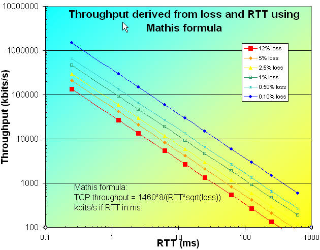
In the above chart the lines are colored according to the packet loss quality defined in Tutorial on Internet Monitoring. Given the difficulty of reducing the RTT, the importance of minimizing packet loss is apparent.
If we consider how the packet loss is improving month-to-month (see Tutorial on Internet monitoring at SLAC) then the loss appears to be improving by between 2% and 9% / month. Applying the above formula, fixing the RTT at 100 msec. and starting with an initial loss of 2.5% we get the throughputs shown in the following figure for various values from 0% to 10% improvement/month:
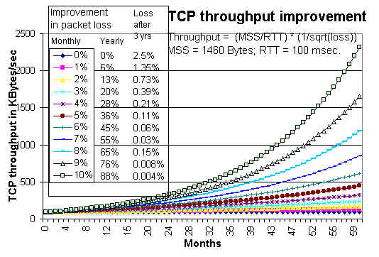
In order to facilitate understanding, the table on the left of the chart above, shows the yearly improvement in loss and the loss at the end of three years.
Using the formula with long term PingER data
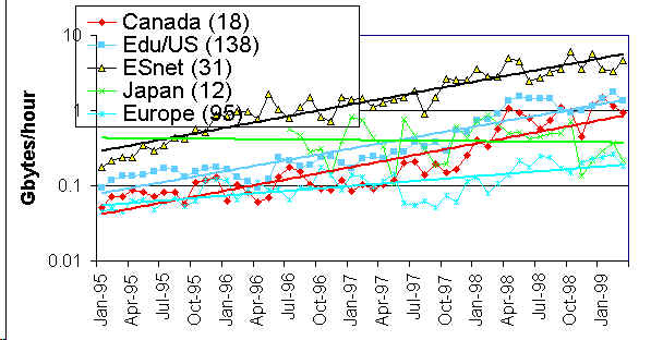
Given the historical measurements from PingER of the packet loss and RTT we can calculate the maximum TCP bandwidth for the last few years for various groups of sites as shown in the figure below. The numbers in parentheses in the legend indicate the number of pairs of monitor-remote sites included in the group measurement. The percentages to the right show the improvement per month, and the straight lines are exponential fits to the data.
Another way of looking at the data is to show the Gbytes that can be transmitted per hour. This is shown in the chart below between ESnet and various collections of sites.
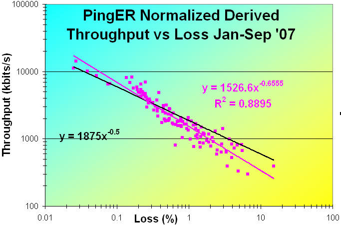
The figure below shows the Normalized Derived PingER Throughput measured from SLAC to countries of the world from january through September 2007 as a function of the packet loss. Normalization is of the form:
Normalized Derived TCP throughput(AKA Normalized Rate) = (Minimum_RTT(Remote country)/Minimum_RTT(Monitoring Country)) * Rate
The correlation is seen to be strong with R2 ~ 0.89, and goes as 1526.6 / loss0.66. Also shown is a rough fit for the 129 countries with observed data minimizing X=Sum(Theory-Observation)/Theory)2) where Theory = beta/sqrt(loss), beta = 1875 and X= 12.43.
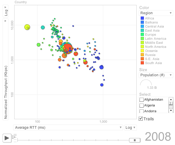
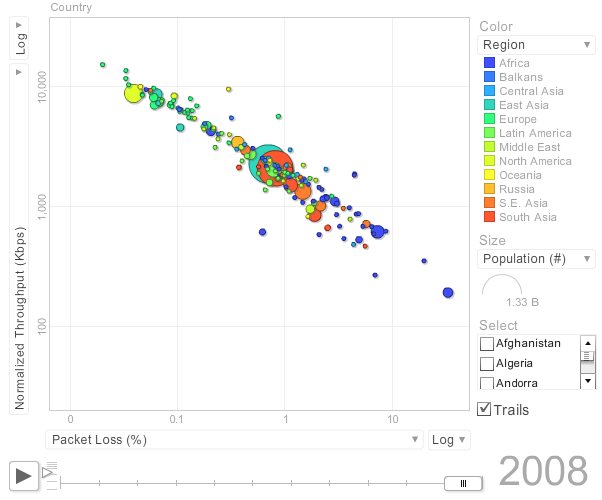
Correlation of Derived Throughput vs Average RTT and Loss
The correlation of Derived Throughput is stronger versus Loss than versus Average RTT. This can be seen in the images below:
| Derived Throughput vs Average RTT | Derived Throughput vs Loss |
|---|---|
|
|
|
[ Feedback | Reporting Problems ]


 1050
1050

 被折叠的 条评论
为什么被折叠?
被折叠的 条评论
为什么被折叠?
 到【灌水乐园】发言


