


EM是我一直想深入学习的算法之一,第一次听说是在NLP课中的HMM那一节,为了解决HMM的参数估计问题,使用了EM算法。在之后的MT中的词对齐中也用到了。在Mitchell的书中也提到EM可以用于贝叶斯网络中。
下面主要介绍EM的整个推导过程。
1. Jensen不等式
回顾优化理论中的一些概念。设f是定义域为实数的函数,如果对于所有的实数x,![]() ,那么f是凸函数。当x是向量时,如果其hessian矩阵H是半正定的(
,那么f是凸函数。当x是向量时,如果其hessian矩阵H是半正定的(![]() ),那么f是凸函数。如果
),那么f是凸函数。如果![]() 或者
或者![]() ,那么称f是严格凸函数。
,那么称f是严格凸函数。
Jensen不等式表述如下:
如果f是凸函数,X是随机变量,那么
![]()
特别地,如果f是严格凸函数,那么![]() 当且仅当
当且仅当![]() ,也就是说X是常量。
,也就是说X是常量。
这里我们将![]() 简写为
简写为![]() 。
。
如果用图表示会很清晰:
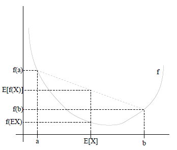
图中,实线f是凸函数,X是随机变量,有0.5的概率是a,有0.5的概率是b。(就像掷硬币一样)。X的期望值就是a和b的中值了,图中可以看到![]() 成立。
成立。
当f是(严格)凹函数当且仅当-f是(严格)凸函数。
Jensen不等式应用于凹函数时,不等号方向反向,也就是![]() 。
。
2. EM算法
给定的训练样本是![]() ,样例间独立,我们想找到每个样例隐含的类别z,能使得p(x,z)最大。p(x,z)的最大似然估计如下:
,样例间独立,我们想找到每个样例隐含的类别z,能使得p(x,z)最大。p(x,z)的最大似然估计如下:

第一步是对极大似然取对数,第二步是对每个样例的每个可能类别z求联合分布概率和。但是直接求![]() 一般比较困难,因为有隐藏变量z存在,但是一般确定了z后,求解就容易了。
一般比较困难,因为有隐藏变量z存在,但是一般确定了z后,求解就容易了。
EM是一种解决存在隐含变量优化问题的有效方法。竟然不能直接最大化![]() ,我们可以不断地建立
,我们可以不断地建立![]() 的下界(E步),然后优化下界(M步)。这句话比较抽象,看下面的。
的下界(E步),然后优化下界(M步)。这句话比较抽象,看下面的。
对于每一个样例i,让![]() 表示该样例隐含变量z的某种分布,
表示该样例隐含变量z的某种分布,![]() 满足的条件是
满足的条件是![]() 。(如果z是连续性的,那么
。(如果z是连续性的,那么![]() 是概率密度函数,需要将求和符号换做积分符号)。比如要将班上学生聚类,假设隐藏变量z是身高,那么就是连续的高斯分布。如果按照隐藏变量是男女,那么就是伯努利分布了。
是概率密度函数,需要将求和符号换做积分符号)。比如要将班上学生聚类,假设隐藏变量z是身高,那么就是连续的高斯分布。如果按照隐藏变量是男女,那么就是伯努利分布了。
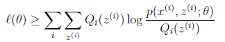
可以由前面阐述的内容得到下面的公式:

(1)到(2)比较直接,就是分子分母同乘以一个相等的函数。(2)到(3)利用了Jensen不等式,考虑到![]() 是凹函数(二阶导数小于0),而且
是凹函数(二阶导数小于0),而且

就是![]() 的期望(回想期望公式中的Lazy Statistician规则)
的期望(回想期望公式中的Lazy Statistician规则)
| 设Y是随机变量X的函数 (1) X是离散型随机变量,它的分布律为 (2) X是连续型随机变量,它的概率密度为 |

对应于上述问题,Y是![]() ,X是
,X是![]() ,
,![]() 是
是![]() ,g是
,g是![]() 到
到![]() 的映射。这样解释了式子(2)中的期望,再根据凹函数时的Jensen不等式:
的映射。这样解释了式子(2)中的期望,再根据凹函数时的Jensen不等式:

可以得到(3)。
这个过程可以看作是对![]() 求了下界。对于
求了下界。对于![]() 的选择,有多种可能,那种更好的?假设
的选择,有多种可能,那种更好的?假设![]() 已经给定,那么
已经给定,那么![]() 的值就决定于
的值就决定于![]() 和
和![]() 了。我们可以通过调整这两个概率使下界不断上升,以逼近
了。我们可以通过调整这两个概率使下界不断上升,以逼近![]() 的真实值,那么什么时候算是调整好了呢?当不等式变成等式时,说明我们调整后的概率能够等价于
的真实值,那么什么时候算是调整好了呢?当不等式变成等式时,说明我们调整后的概率能够等价于![]() 了。按照这个思路,我们要找到等式成立的条件。根据Jensen不等式,要想让等式成立,需要让随机变量变成常数值,这里得到:
了。按照这个思路,我们要找到等式成立的条件。根据Jensen不等式,要想让等式成立,需要让随机变量变成常数值,这里得到:

c为常数,不依赖于![]() 。对此式子做进一步推导,我们知道
。对此式子做进一步推导,我们知道![]() ,那么也就有
,那么也就有![]() ,(多个等式分子分母相加不变,这个认为每个样例的两个概率比值都是c),那么有下式:
,(多个等式分子分母相加不变,这个认为每个样例的两个概率比值都是c),那么有下式:

至此,我们推出了在固定其他参数![]() 后,
后,![]() 的计算公式就是后验概率,解决了
的计算公式就是后验概率,解决了![]() 如何选择的问题。这一步就是E步,建立
如何选择的问题。这一步就是E步,建立![]() 的下界。接下来的M步,就是在给定
的下界。接下来的M步,就是在给定![]() 后,调整
后,调整![]() ,去极大化
,去极大化![]() 的下界(在固定
的下界(在固定![]() 后,下界还可以调整的更大)。那么一般的EM算法的步骤如下:
后,下界还可以调整的更大)。那么一般的EM算法的步骤如下:
| 循环重复直到收敛 { (E步)对于每一个i,计算 (M步)计算 |

那么究竟怎么确保EM收敛?假定![]() 和
和![]() 是EM第t次和t+1次迭代后的结果。如果我们证明了
是EM第t次和t+1次迭代后的结果。如果我们证明了![]() ,也就是说极大似然估计单调增加,那么最终我们会到达最大似然估计的最大值。下面来证明,选定
,也就是说极大似然估计单调增加,那么最终我们会到达最大似然估计的最大值。下面来证明,选定![]() 后,我们得到E步
后,我们得到E步
![]()
这一步保证了在给定![]() 时,Jensen不等式中的等式成立,也就是
时,Jensen不等式中的等式成立,也就是
然后进行M步,固定![]() ,并将
,并将![]() 视作变量,对上面的
视作变量,对上面的![]() 求导后,得到
求导后,得到![]() ,这样经过一些推导会有以下式子成立:
,这样经过一些推导会有以下式子成立:
解释第(4)步,得到![]() 时,只是最大化
时,只是最大化![]() ,也就是
,也就是![]() 的下界,而没有使等式成立,等式成立只有是在固定
的下界,而没有使等式成立,等式成立只有是在固定![]() ,并按E步得到
,并按E步得到![]() 时才能成立。
时才能成立。
况且根据我们前面得到的下式,对于所有的![]() 和
和![]() 都成立
都成立
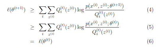
第(5)步利用了M步的定义,M步就是将![]() 调整到
调整到![]() ,使得下界最大化。因此(5)成立,(6)是之前的等式结果。
,使得下界最大化。因此(5)成立,(6)是之前的等式结果。
这样就证明了![]() 会单调增加。一种收敛方法是
会单调增加。一种收敛方法是![]() 不再变化,还有一种就是变化幅度很小。
不再变化,还有一种就是变化幅度很小。
再次解释一下(4)、(5)、(6)。首先(4)对所有的参数都满足,而其等式成立条件只是在固定![]() ,并调整好Q时成立,而第(4)步只是固定Q,调整
,并调整好Q时成立,而第(4)步只是固定Q,调整![]() ,不能保证等式一定成立。(4)到(5)就是M步的定义,(5)到(6)是前面E步所保证等式成立条件。也就是说E步会将下界拉到与
,不能保证等式一定成立。(4)到(5)就是M步的定义,(5)到(6)是前面E步所保证等式成立条件。也就是说E步会将下界拉到与![]() 一个特定值(这里
一个特定值(这里![]() )一样的高度,而此时发现下界仍然可以上升,因此经过M步后,下界又被拉升,但达不到与
)一样的高度,而此时发现下界仍然可以上升,因此经过M步后,下界又被拉升,但达不到与![]() 另外一个特定值一样的高度,之后E步又将下界拉到与这个特定值一样的高度,重复下去,直到最大值。
另外一个特定值一样的高度,之后E步又将下界拉到与这个特定值一样的高度,重复下去,直到最大值。
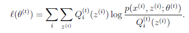
如果我们定义
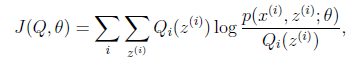
从前面的推导中我们知道![]() ,EM可以看作是J的坐标上升法,E步固定
,EM可以看作是J的坐标上升法,E步固定![]() ,优化
,优化![]() ,M步固定
,M步固定![]() 优化
优化![]() 。
。
3. 重新审视混合高斯模型
我们已经知道了EM的精髓和推导过程,再次审视一下混合高斯模型。之前提到的混合高斯模型的参数![]() 和
和![]() 计算公式都是根据很多假定得出的,有些没有说明来由。为了简单,这里在M步只给出
计算公式都是根据很多假定得出的,有些没有说明来由。为了简单,这里在M步只给出![]() 和
和![]() 的推导方法。
的推导方法。
E步很简单,按照一般EM公式得到:
![]()
简单解释就是每个样例i的隐含类别![]() 为j的概率可以通过后验概率计算得到。
为j的概率可以通过后验概率计算得到。
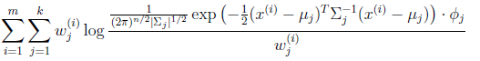
在M步中,我们需要在固定![]() 后最大化最大似然估计,也就是
后最大化最大似然估计,也就是

这是将![]() 的k种情况展开后的样子,未知参数
的k种情况展开后的样子,未知参数![]() 和
和![]() 。
。
固定![]() 和
和![]() ,对
,对![]() 求导得
求导得

等于0时,得到
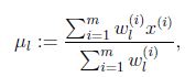
这就是我们之前模型中的![]() 的更新公式。
的更新公式。
然后推导![]() 的更新公式。看之前得到的
的更新公式。看之前得到的
在![]() 和
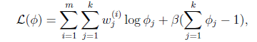
和![]() 确定后,分子上面的一串都是常数了,实际上需要优化的公式是:
确定后,分子上面的一串都是常数了,实际上需要优化的公式是:
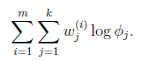
需要知道的是,![]() 还需要满足一定的约束条件就是
还需要满足一定的约束条件就是![]() 。
。
这个优化问题我们很熟悉了,直接构造拉格朗日乘子。
还有一点就是![]() ,但这一点会在得到的公式里自动满足。
,但这一点会在得到的公式里自动满足。
求导得,
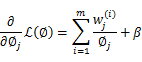
等于0,得到

也就是说![]() 再次使用
再次使用![]() ,得到
,得到
![]()
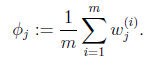
这样就神奇地得到了![]() 。
。
那么就顺势得到M步中![]() 的更新公式:
的更新公式:
![]() 的推导也类似,不过稍微复杂一些,毕竟是矩阵。结果在之前的混合高斯模型中已经给出。
的推导也类似,不过稍微复杂一些,毕竟是矩阵。结果在之前的混合高斯模型中已经给出。
4. 总结
如果将样本看作观察值,潜在类别看作是隐藏变量,那么聚类问题也就是参数估计问题,只不过聚类问题中参数分为隐含类别变量和其他参数,这犹如在x-y坐标系中找一个曲线的极值,然而曲线函数不能直接求导,因此什么梯度下降方法就不适用了。但固定一个变量后,另外一个可以通过求导得到,因此可以使用坐标上升法,一次固定一个变量,对另外的求极值,最后逐步逼近极值。对应到EM上,E步估计隐含变量,M步估计其他参数,交替将极值推向最大。EM中还有“硬”指定和“软”指定的概念,“软”指定看似更为合理,但计算量要大,“硬”指定在某些场合如K-means中更为实用(要是保持一个样本点到其他所有中心的概率,就会很麻烦)。
另外,EM的收敛性证明方法确实很牛,能够利用log的凹函数性质,还能够想到利用创造下界,拉平函数下界,优化下界的方法来逐步逼近极大值。而且每一步迭代都能保证是单调的。最重要的是证明的数学公式非常精妙,硬是分子分母都乘以z的概率变成期望来套上Jensen不等式,前人都是怎么想到的。
在Mitchell的Machine Learning书中也举了一个EM应用的例子,明白地说就是将班上学生的身高都放在一起,要求聚成两个类。这些身高可以看作是男生身高的高斯分布和女生身高的高斯分布组成。因此变成了如何估计每个样例是男生还是女生,然后在确定男女生情况下,如何估计均值和方差,里面也给出了公式,有兴趣可以参考。


 4056
4056

 被折叠的 条评论
为什么被折叠?
被折叠的 条评论
为什么被折叠?
 到【灌水乐园】发言


