算法时间复杂度和空间复杂度

最新推荐文章于 2021-07-04 22:16:22 发布

置顶不懂不想说

最新推荐文章于 2021-07-04 22:16:22 发布

阅读量6.2k

点赞数

分类专栏：算法文章标签：算法

算法专栏收录该内容

21 篇文章 1 订阅

订阅专栏

定义

空间复杂度(Space Complexity)是对一个算法在运行过程中临时占用存储空间大小的量度,记做S(n)=O(f(n))。比如直接插入排序的时间复杂度是O(n^2), 空间复杂度是O(1) 。而一般的递归算法就要有O(n)的空间复杂度了,因为每次递归都要存储返回信息。一个算法的优劣主要从算法的执行时间和所需要占用的存储空间两个方面衡量。

编辑本段 空间复杂度

类似于时间复杂度的讨论，一个算法的空间复杂度(SpaceComplexity)S(n)定义为该算法所耗费的存储空间，它也是问题规模n的函数。渐近空间复杂度也常常简称为空间复杂度。空间复杂度(SpaceComplexity)是对一个算法在运行过程中临时占用存储空间大小的量度。一个算法在计算机存储器上所占用的存储空间，包括存储算法本身所占用的存储空间，算法的输入输出数据所占用的存储空间和算法在运行过程中临时占用的存储空间这三个方面。算法的输入输出数据所占用的存储空间是由要解决的问题决定的，是通过参数表由调用函数传递而来的，它不随本算法的不同而改变。存储算法本身所占用的存储空间与算法书写的长短成正比，要压缩这方面的存储空间，就必须编写出较短的算法。算法在运行过程中临时占用的存储空间随算法的不同而异，有的算法只需要占用少量的临时工作单元，而且不随问题规模的大小而改变，我们称这种算法是“就地\"进行的，是节省存储的算法，如这一节介绍过的几个算法都是如此；有的算法需要占用的临时工作单元数与解决问题的规模n有关，它随着n的增大而增大，当n较大时，将占用较多的存储单元，例如将在第九章介绍的快速排序和归并排序算法就属于这种情况。

分析一个算法所占用的存储空间要从各方面综合考虑。如对于递归算法来说，一般都比较简短，算法本身所占用的存储空间较少，但运行时需要一个附加堆栈，从而占用较多的临时工作单元；若写成非递归算法，一般可能比较长，算法本身占用的存储空间较多，但运行时将可能需要较少的存储单元。

一个算法的空间复杂度只考虑在运行过程中为局部变量分配的存储空间的大小，它包括为参数表中形参变量分配的存储空间和为在函数体中定义的局部变量分配的存储空间两个部分。若一个算法为递归算法，其空间复杂度为递归所使用的堆栈空间的大小，它等于一次调用所分配的临时存储空间的大小乘以被调用的次数(即为递归调用的次数加1，这个1表示开始进行的一次非递归调用)。算法的空间复杂度一般也以数量级的形式给出。如当一个算法的空间复杂度为一个常量，即不随被处理数据量n的大小而改变时，可表示为O(1)；当一个算法的空间复杂度与以2为底的n的对数成正比时，可表示为O(log2n)；当一个算法的空I司复杂度与n成线性比例关系时，可表示为O(n).若形参为数组，则只需要为它分配一个存储由实参传送来的一个地址指针的空间，即一个机器字长空间；若形参为引用方式，则也只需要为其分配存储一个地址的空间，用它来存储对应实参变量的地址，以便由系统自动引用实参变量。

编辑本段 时间与空间复杂度比较

对于一个算法，其时间复杂度和空间复杂度往往是相互影响的。当追求一个较好的时间复杂度时，可能会使空间复杂度的性能变差，即可能导致占用较多的存储空间；反之，当追求一个较好的空间复杂度时，可能会使时间复杂度的性能变差，即可能导致占用较长的运行时间。另外，算法的所有性能之间都存在着或多或少的相互影响。因此，当设计一个算法(特别是大型算法)时，要综合考虑算法的各项性能，算法的使用频率，算法处理的数据量的大小，算法描述语言的特性，算法运行的机器系统环境等各方面因素，才能够设计出比较好的算法。算法的时间复杂度和空间复杂度合称为算法的复杂度。

在计算机科学中，算法的时间复杂度是一个函数，它定量描述了该算法的运行时间。这是一个关于代表算法输入值的字符串的长度的函数。时间复杂度常用大O符号表述，不包括这个函数的低阶项和首项系数。使用这种方式时，时间复杂度可被称为是渐近的，它考察当输入值大小趋近无穷时的情况。举例，如果一个算法对于任何大小为 $n$ 的输入，它至多需要 $5n^3+3n$ 的时间运行完毕，那么它的渐近时间复杂度是 $O(n^3)$ 。

计算时间复杂度的过程，常常需要分析一个算法运行过程中需要的基本操作，计量所有操作的数量。通常假设一个基本操作可在固定时间内完成，因此总运行时间和操作的总数量最多相差一个常量系数。

有时候，即使对于大小相同的输入，同一算法的效率也可能不同。因此，常对最坏时间复杂度进行分析。最坏时间复杂度定义为对于给定大小 $n$ 的任何输入，某个算法的最大运行时间，记为 $T(n)$ 。通常根据 $T(n)$ 对时间复杂度进行分类。比如，如果对某个算法有 $T(n) = O(n)$ ，则称其具有线性时间。如有 $T(n) = O(2^n)$ ，则称其具有指数时间。

常见时间复杂度列表[编辑]

更多资料：数学运算的计算复杂度

以下是一些常见时间复杂度的例子。

名称	复杂度类	运行时间（ $T(n)$ ）	运行时间举例	算法举例
常数时间		$O(1)$	10	判断一个二进制数的奇偶
反阿克曼时间		$O(\alpha(n))$		并查集的单个操作的平摊时间
迭代对数时间		$O(\log^{*}n)$		en:Cole-Vishkin algorithm
对数对数时间		$O(\log \log n)$		有界优先队列的单个操作^[1]
对数时间	DLOGTIME	$O(\log n)$	$\log n$ ， $\log n^2$	二分搜索
幂对数时间		$(\log n)^{O(1)}$	$(\log n)^2$
（小于1次）幂时间		$O(n^c)$ ，其中 $0 < c < 1$	$n^{\frac{1}{2}}$ ， $n^{\frac{2}{3}}$	K-d树的搜索操作
线性时间		$O(n)$	$n$	无序数组的搜索
线性迭代对数时间		$O(n\log^{*}n)$		Raimund Seidel（英语：Raimund Seidel）的三角分割多边形（英语：Polygon triangulation）算法
线性对数时间		$O(n\log n)$	$n\log n$ ， $n \log n!$	最快的比较排序
二次时间		$O(n^2)$	$n^2$	冒泡排序、插入排序
三次时间		$O(n^3)$	$n^3$	矩阵乘法的基本实现，计算部分相关性（英语：Partial correlation）
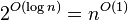多项式时间	P	$2^{O(\log n)} = n^{O(1)}$	$n$ ， $n \log n$ ， $n^{10}$	线性规划中的en:Karmarkar's algorithm， AKS质数测试
准多项式时间	QP	$2^{(\log n)^{O(1)}}$	$n^{\log \log n}$ ， $n^{\log n}$	关于有向斯坦纳树问题（英语：Steiner tree problem）最著名的 $O(\log^2 n)$ 近似算法
次指数时间（第一定义）	SUBEXP	$O^{2^{n^{\epsilon}}}$ ，对任意的 ε > 0	$O(2^{(\log n)^{\log \log n}})$	Assuming complexity theoretic conjectures, BPP is contained in SUBEXP.^[2]
次指数时间（第二定义）		2^o(n)	2^{n^1/3}	Best-known algorithm for integer factorization and graph isomorphism
指数时间	E	2^O(n)	1.1ⁿ, 10ⁿ	使用动态规划解决旅行推销员问题
阶乘时间		O(n!)	n!	通过暴力搜索解决旅行推销员问题
exponential time	EXPTIME	2^poly(n)	2ⁿ, 2^n²
double exponential time	2-EXPTIME	2^{2^poly(n)}	2^2ⁿ	Deciding the truth of a given statement in Presburger arithmetic

常数时间[编辑]

主条目：常数时间

若对于一个算法， $T(n)$ 的上界与输入大小无关，则称其具有常数时间，记作 $O(1)$ 时间。一个例子是访问数组中的单个元素，因为访问它只需要一条指令。但是，找到无序数组中的最小元素则不是，因为这需要遍历所有元素来找出最小值。这是一项线性时间的操作，或称 $O(n)$ 时间。但如果预先知道元素的数量并假设数量保持不变，则该操作也可被称为具有常数时间。

虽然被称为“常数时间”，运行时间本身并不必须与问题规模无关，但它的上界必须是与问题规模无关的确定值。举例，“如果 a > b 则交换 a、b 的值”这项操作，尽管具体时间会取决于条件“a > b”是否满足，但它依然是常数时间，因为存在一个常量 t 使得所需时间总不超过 t。

以下是一个常数时间的代码片段：

int index = 5;
int item = list[index];
if (condition true) then
   perform some operation that runs in constant time
else
   perform some other operation that runs in constant time
for i = 1 to 100
   for j = 1 to 200
      perform some operation that runs in constant time

如果 $T(n) = O(c)$ ，其中 $c$ 是一个常数，这记法等价于标准记法 $T(n) = O(1)$ 。

对数时间[编辑]

主条目：对数时间

若算法的 T(n) = O(log n)，则称其具有对数时间。由于计算机使用二进制的记数系统，对数常常以2为底（即log₂n，有时写作 lg n）。然而，由对数的换底公式，log_an 和 log_b n只有一个常数因子不同，这个因子在大O记法中被丢弃。因此记作O(log n)，而不论对数的底是多少，是对数时间算法的标准记法。

常见的具有对数时间的算法有二叉树的相关操作和二分搜索。

A O(log n) algorithm is considered highly efficient, as the operations per instance required to complete decrease with each instance.

A very simple example of this type of f(n) is an algorithm that cuts a string in half. It will take O(log n) time (n being the length of the string) since we chop the string in half before each print. This means, in order to increase the number of prints, we have to double the length of the string.

// 递归输出一个字符串的右半部分
var right = function(str)
{
    var length = str.length;
 
    // 辅助函数
    var help = function(index)
    {
 
        // 递归情况：输出右半部分
        if(index < length){
 
            // 输出从 index 到数组末尾的部分
            console.log(str.substring(index, length));
 
            // 递归调用：调用辅助函数，将右半部分作为参数传入
            help(Math.ceil((length + index)/2));
        }
 
        // 基本情况：什么也不做
    }
    help(0);
}

幂对数时间[编辑]

An algorithm is said to run in polylogarithmic time if T(n) = O((logn)^k), for some constant k. For example, matrix chain ordering can be solved in polylogarithmic time on aParallel Random Access Machine.^[3]

Sub-linear time[编辑]

An algorithm is said to run in sub-linear time (often spelledsublinear time) if T(n) = o(n). In particular this includes algorithms with the time complexities defined above, as well as others such as the O(n^½)Grover's search algorithm.

Typical algorithms that are exact and yet run in sub-linear time use parallel processing (as the NC₁ matrix determinant calculation does),non-classical processing (as Grover's search does), or alternatively have guaranteed assumptions on the input structure (as the logarithmic timebinary search and many tree maintenance algorithms do). However, languages such as the set of all strings that have a 1-bit indexed by the first log(n) bits may depend on every bit of the input and yet be computable in sub-linear time.

The specific term sublinear time algorithm is usually reserved to algorithms that are unlike the above in that they are run over classical serial machine models and are not allowed prior assumptions on the input.^[4] They are however allowed to be randomized, and indeed must be randomized for all but the most trivial of tasks.

As such an algorithm must provide an answer without reading the entire input, its particulars heavily depend on the access allowed to the input. Usually for an input that is represented as a binary stringb₁,...,b_k it is assumed that the algorithm can in time O(1) request and obtain the value ofb_i for any i.

Sub-linear time algorithms are typically randomized, and provide only approximate solutions. In fact, the property of a binary string having only zeros (and no ones) can be easily proved not to be decidable by a (non-approximate) sub-linear time algorithm. Sub-linear time algorithms arise naturally in the investigation ofproperty testing.

线性时间[编辑]

如果一个算法的时间复杂度为O(n)，则称这个算法具有线性时间，或 O(n) 时间。非正式地说，这意味着对于足够大的输入，运行时间增加的大小与输入成线性关系。例如,一个计算列表所有元素的和的程序，需要的时间与列表的长度成正比。这个描述是稍微不准确的，因为运行时间可能显著偏离一个精确的比例，尤其是对于较小的n。

Linear time is often viewed as a desirable attribute for an algorithm. Much research has been invested into creating algorithms exhibiting (nearly) linear time or better. This research includes both software and hardware methods. In the case of hardware, some algorithms which, mathematically speaking, can never achieve linear time with standardcomputation models are able to run in linear time. There are several hardware technologies which exploitparallelism to provide this. An example is content-addressable memory. This concept of linear time is used in string matching algorithms such as theBoyer-Moore Algorithm and Ukkonen's Algorithm.

线性对数（准线性）时间[编辑]

A linearithmic function (portmanteau oflinear and logarithmic) is a function of the form n · logn (i.e., a product of a linear and a logarithmic term). An algorithm is said to run in linearithmic time ifT(n) = O(n log n). Compared to other functions, a linearithmic function is ω(n), o(n^1+ε) for every ε > 0, and Θ(n · logn). Thus, a linearithmic term grows faster than a linear term but slower than any polynomial inn with exponent strictly greater than 1.

An algorithm is said to run in quasilinear time if T(n) =O(n log^k n) for any constantk. Quasilinear time algorithms are also o(n^1+ε) for every ε > 0, and thus run faster than any polynomial inn with exponent strictly greater than 1.

In many cases, the n · log n running time is simply the result of performing a Θ(logn) operation n times. For example, binary tree sort creates a binary tree by inserting each element of the n-sized array one by one. Since the insert operation on aself-balancing binary search tree takes O(log n) time, the entire algorithm takes linearithmic time.

比较排序s require at least linearithmic number of comparisons in the worst case because log(n!) = Θ(n logn), by Stirling's approximation. They also frequently arise from the recurrence relation T(n) = 2 T(n/2) + O(n).

Some famous algorithms that run in linearithmic time include:

Comb sort, in theaverage and worst case
Quicksort in the average case
Heapsort,merge sort, introsort, binary tree sort, smoothsort, patience sorting, etc. in the worst case
Fast Fourier transforms
Monge array calculation

Sub-quadratic time[编辑]

An algorithm is said to be subquadratic time if T(n) = o(n²).

For example, most naïve comparison-based sorting algorithms are quadratic (e.g. insertion sort), but more advanced algorithms can be found that are subquadratic (e.g.Shell sort). No general-purpose sorts run in linear time, but the change from quadratic to sub-quadratic is of great practical importance.

多项式时间[编辑]

An algorithm is said to be of polynomial time if its running time isupper bounded by a polynomial expression in the size of the input for the algorithm, i.e., T(n) = O(n^k) for some constantk.^[5]^[6]Problems for which a polynomial time algorithm exists belong to the complexity class P, which is central in the field ofcomputational complexity theory. Cobham's thesis states that polynomial time is a synonym for "tractable", "feasible", "efficient", or "fast".^[7]

Some examples of polynomial time algorithms:

The quicksort sorting algorithm on n integers performs at most $An^2$ operations for some constantA. Thus it runs in time $O(n^2)$ and is a polynomial time algorithm.
All the basic arithmetic operations (addition, subtraction, multiplication, division, and comparison) can be done in polynomial time.
Maximum matchings ingraphs can be found in polynomial time.

强多项式时间与弱多项式时间[编辑]

In some contexts, especially in optimization, one differentiates between strongly polynomial time andweakly polynomial time algorithms. These two concepts are only relevant if the inputs to the algorithms consist of integers.

Strongly polynomial time is defined in the arithmetic model of computation. In this model of computation the basic arithmetic operations (addition, subtraction, multiplication, division, and comparison) take a unit time step to perform, regardless of the sizes of the operands. The algorithm runs in strongly polynomial time if ^[8]

the number of operations in the arithmetic model of computation is bounded by a polynomial in the number of integers in the input instance; and
the space used by the algorithm is bounded by a polynomial in the size of the input.

Any algorithm with these two properties can be converted to a polynomial time algorithm by replacing the arithmetic operations by suitable algorithms for performing the arithmetic operations on aTuring machine. If the second of the above requirement is not met, then this is not true anymore. Given the integer $2^n$ (which takes up space proportional to n), it is possible to compute $2^{2^n}$ with n multiplications usingrepeated squaring. However, the space used to represent $2^{2^n}$ is proportional to $2^n$ , and thus exponential rather than polynomial in the space used to represent the input. Hence, it is not possible to carry out this computation in polynomial time on a Turing machine, but it is possible to compute it by polynomially many arithmetic operations.

Conversely, there are algorithms which run in a number of Turing machine steps bounded by a polynomial in the length of binary-encoded input, but do not take a number of arithmetic operations bounded by a polynomial in the number of input numbers. TheEuclidean algorithm for computing the greatest common divisor of two integers is one example. Given two integers $a$ and $b$ the running time of the algorithm is bounded by $O((\log\ a + \log\ b)^2)$ Turing machine steps. This is polynomial in the size of a binary representation of $a$ and $b$ as the size of such a representation is roughly $\log\ a + \log\ b$ . At the same time, the number of arithmetic operations cannot be bound by the number of integers in the input (which is constant in this case, there is always only two integers in the input). Due to the latter observation, the algorithm does not run in strongly polynomial time. Its real running time depends on the magnitudes of $a$ and $b$ and not only on the number of integers in the input.

An algorithm which runs in polynomial time but which is not strongly polynomial is said to run inweakly polynomial time.^[9] A well-known example of a problem for which a weakly polynomial-time algorithm is known, but is not known to admit a strongly polynomial-time algorithm, islinear programming. Weakly polynomial-time should not be confused with pseudo-polynomial time.

空间复杂度：

编辑本段 时间与空间复杂度比较

不懂不想说

关注

0
点赞
踩
6

收藏

觉得还不错? 一键收藏
0
评论
算法时间复杂度和空间复杂度

定义空间复杂度(Space Complexity)是对一个算法在运行过程中临时占用存储空间大小的量度,记做S(n)=O(f(n))。比如直接插入排序的时间复杂度是O(n^2),空间复杂度是O(1) 。而一般的递归算法就要有O(n)的空间复杂度了,因为每次递归都要存储返回信息。一个算法的优劣主要从算法的执行时间和所需要占用的存储空间两个方面衡量。编辑本段空间复杂度类似于时间复杂度的讨
复制链接

扫一扫

专栏目录