


问题:
以下查询涉及 90 行,只占总行数的 90/10000 ,但使用了全表扫描:
select /*+ gather_plan_statistics */ count ( distinct junk ), count (*)
    from  bricks
    where  weight between 1 and 10;
   COUNT(DISTINCTJUNK)    COUNT(*)
______________________ ___________
     4          90

-------------------------------------------------------------------------------------------
| Id  | Operation     | Name| Starts | E-Rows | A-Rows |   A-Time| Buffers |
-------------------------------------------------------------------------------------------
|   0 | SELECT STATEMENT     ||      1 |  | 1 |00:00:00.01 |     120 |
|   1 |  SORT AGGREGATE      ||      1 |1 | 1 |00:00:00.01 |     120 |
|   2 |   VIEW         |      VW_DAG_0 |  1 | 92 | 4 |00:00:00.01 |     120 |
|   3 |    HASH GROUP BY     ||      1 |     92 | 4 |00:00:00.01 |     120 |
|*  4 |     TABLE ACCESS FULL| BRICKS|      1 |     92 |90 |00:00:00.01 |     120 |
-------------------------------------------------------------------------------------------
Predicate Information (identified by operation id):
---------------------------------------------------
   4 - filter(("WEIGHT"<=10 AND "WEIGHT">=1))
22 rows selected.
以下查询涉及 1000 行,反而使用了索引:
select /*+ gather_plan_statistics */ count ( distinct junk ), count (*)
    from  bricks
    where  brick_id between 1 and 1000;

COUNT(DISTINCTJUNK)   COUNT(*)
------------------- ----------
  4         1000
为什么涉及行数少的查询,反而不走索引了?
------------------------------------------------------------------------------------------------------
| Id  | Operation       | Name   | Starts | E-Rows | A-Rows |   A-Time   | Buffers |
------------------------------------------------------------------------------------------------------
|   0 | SELECT STATEMENT       |   |  1 |     |    1 |00:00:00.01 |  15 |
|   1 |  SORT AGGREGATE        |   |  1 |   1 |    1 |00:00:00.01 |  15 |
|   2 |   VIEW       | VW_DAG_0  |  1 | 995 |    4 |00:00:00.01 |  15 |
|   3 |    HASH GROUP BY       |   |  1 | 995 |    4 |00:00:00.01 |  15 |
|   4 |     TABLE ACCESS BY INDEX ROWID| BRICKS    |  1 | 995 | 1000 |00:00:00.01 |  15 |
|*  5 |      INDEX RANGE SCAN       | BRICKS_PK |  1 | 995 | 1000 |00:00:00.01 |   3 |
------------------------------------------------------------------------------------------------------
Predicate Information (identified by operation id):
---------------------------------------------------
   5 - access("BRICK_ID">=1 AND "BRICK_ID"<=1000)
23 rows selected.
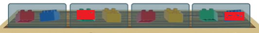
下面用不同颜色的积木表示数据,存放积木的盒子表示数据块。
下面我们有 4 个数据块,存储了不同颜色的积木,每个盒子有 2 个积木,下面需要找出红色积木 :
select * from bricks where colour = 'red';
全表扫描方式:
-
读取表中所有块。
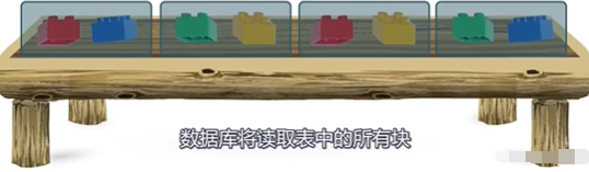
-
逐个块进行查找,选出符合条件的数据。

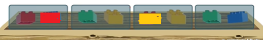
索引扫描方式
只扫描存在红色积木的盒子,而不是所有盒子。


使用索引时数据库访问多少数据块,取决于这些行在表中的物理位置
在使用索引时,存在两个极端情况
-
需要查询的数据,全都位于同一个数据块内。
例如红色积木,在同一个盒子里,在索引扫描查询红色积木时,只需要查 1 个盒子,即 1 次 I/O 。
-
需要查询的每条数据,全都分散在不同的数据库内。
红色积木,分布在不同的盒子里。在索引扫描查询红色积木时,只需要两个盒子,即 2 次 I/O 。
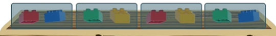
或者每个盒子都只有一个红积木,此时查询红色积木需要查找 5 个盒子,即 5 次 I/O ,接近全面扫描 I/O 次数。
数据库如何知道在运行查询之前使用索引需要访问多少个块呢?
实际上数据库也无法精准计算出数据块个数,但是可以通过聚簇因子来进行评估。
什么是聚簇因子
Oralce 数据库系统中最普通,最为常用的即为堆表。
堆表的数据存储方式为无序存储,也就是任意的DML 操作都可能使得当前数据块存在可用的空闲空间。
处于节省空间的考虑,块上的可用空闲空间会被新插入的行填充,而不是按顺序填充到最后被使用的块上。
上述的操作方式导致了数据的无序性的产生。
当创建索引时,会根据指定的列按顺序来填充到索引块,缺省的情况下为升序。
新建或重建索引时,索引列上的顺序是有序的,而表上的顺序是无序的,也就是存在了差异,即表现为聚簇因子。
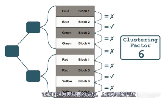
聚簇因子是数据库在收集表统计信息时计算得出的一个计算器。
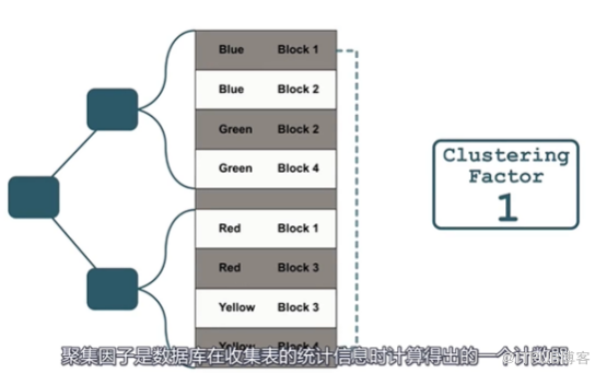
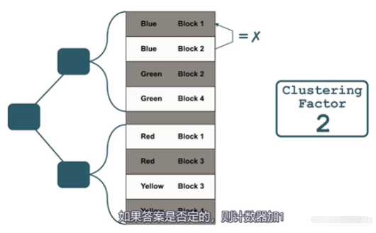
它会统计当前数据是否和上一条数据在同一个块中。
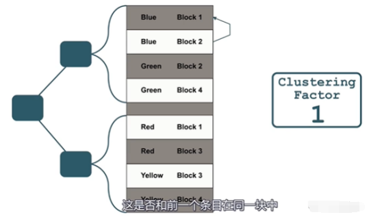
如果不在一个块中,聚簇因子计算加 1 。
如果在同一个块中,计数器保持不变。

所以聚簇因子的下限是表的块数,上限是表的行数。
块数 <= 聚簇因子 <= 行数
聚簇因子越高,索引中的顺序行在整个表中的分散度越高,索引效率可能越低。
聚簇因子是基于表上索引列上的一个值,每一个索引都有一个聚簇因子。
用于描述索引块上与表块上存储数据在顺序上的相似程度,也就说表上的数据行的存储顺序与索引列上顺序是否一致。
在全索引扫描中, CF 的值基本上等同于物理 I/O 或块访问数,如果相同的块被连续读,则 Oracle 认为只需要 1 次物理 I/O 。
好的 CF 值接近于表上的块数,而差的 CF 值则接近于表上的行数。
聚簇因子在索引创建时就会通过表上存存在的行以及索引块计算获得
Oracle 如何计算聚簇因子
执行或预估一次全索引扫描。
检查索引块上每一个rowid 的值,查看是否前一个 rowid 的值与后一个指向了相同的数据块,如果指向了不相同的数据块则 CF 的值增加 1 。
当索引块上的每一个rowid 被检查完毕,即得到最终的 CF 值。
这也就是为什么在最开始的两个 SQL ,查询行数少的为什么不走索引,还是因为聚簇因子的原因。
实验
下面通过实验来看下聚簇因子的影响
创建环境
创建表bricks和索引,及全局临时表bricks_temp,并在最后搜集统计信息:
conn cjc/******
复位随机数
exec dbms_random.seed ( 0 );
创建表bricks,
create table bricks (
  brick_id not null constraint bricks_pk primary key,
  colour   not null,
  shape    not null,
  weight   not null,
  insert_date not null,
  junk     default lpad ( 'x', 50, 'x' ) not null
) as
  with rws as (
    select level x from dual
    connect by level <= 10000
  )
    select rownum brick_id,
           case ceil ( rownum / 2500 )
             when 4 then 'red'
             when 1 then 'blue'
             when 2 then 'green'
             when 3 then 'yellow'
           end colour,
           case mod ( rownum, 4 )
             when 0 then 'cube'
             when 1 then 'cylinder'
             when 2 then 'pyramid'
             when 3 then 'prism'
           end shape,
           round ( dbms_random.value ( 1, 1000 ) ),
           date'2022-01-01' + ( rownum/24 ) + ( mod ( rownum, 24 ) / 36 ) insert_date,
           lpad ( ascii ( mod ( rownum, 26 ) + 65 ), 50, 'x' )
    from   rws;
查看表结构
SQL> desc bricks
 Name   Null?    Type
 ----------------------------------------- -------- ----------------------------
 BRICK_ID   NOT NULL NUMBER
 COLOUR    NOT NULL VARCHAR2(6)
 SHAPE   NOT NULL VARCHAR2(8)
 WEIGHT    NOT NULL NUMBER
 INSERT_DATE   NOT NULL DATE
 JUNK   NOT NULL VARCHAR2(200)
创建临时表bricks_temp
create global temporary table bricks_temp as
  select * from bricks
  where  1 = 0;
创建索引,索引列weight
create index brick_weight_i on
  bricks ( weight );
创建索引,索引列shape
create index brick_shape_i on
  bricks ( shape );
创建索引,索引列colour
create index brick_colour_i on
  bricks ( colour );
创建索引,索引列insert_date
create index brick_insert_date_i on
  bricks ( insert_date );
收集表统计信息
EXEC DBMS_STATS.GATHER_TABLE_STATS('CJC','BRICKS',estimate_percent=>100,method_opt=> 'FOR ALL INDEXED COLUMNS',CASCADE=> TRUE);
查看数据,bricks表有10000行:
SQL> select count(*) from bricks;
   COUNT(*)
___________
      10000
查询数据
SQL>
SELECT
    brick_id,
    colour,
    shape,
    weight,
    insert_date
FROM
    bricks
WHERE
    ROWNUM <= 9;

 BRICK_ID COLOUR SHAPE        WEIGHT INSERT_DATE
---------- ------ -------- ---------- ------------------
 1 blue   cylinder   64 01-JAN-22
 2 blue   pyramid  829 01-JAN-22
 3 blue   prism   233 01-JAN-22
 4 blue   cube  219 01-JAN-22
 5 blue   cylinder  371 01-JAN-22
 6 blue   pyramid   70 01-JAN-22
 7 blue   prism   461 01-JAN-22
 8 blue   cube  953 01-JAN-22
 9 blue   cylinder  944 01-JAN-22
9 rows selected.
junk列长度为1000,目的是将行撑大,没有在结果集中显示。
索引什么时候有用?
大家通常认为,当索引定位表中的很少几行时,它被认为是有用的。
但很少有多少?这个很难界定。我们通过示例来了解一下。
bricks表现有5个索引:
set line 300
col cols for a25
select ui.index_name,
       listagg ( uic.column_name, ',' )
         within group ( order by column_position ) cols
from   user_indexes ui
join   user_ind_columns uic
on     ui.index_name = uic.index_name
where  ui.table_name = 'BRICKS'
group  by ui.index_name;
INDEX_NAME       COLS
------------------------------ -------------------------
BRICKS_PK           BRICK_ID
BRICK_COLOUR_I       COLOUR
BRICK_INSERT_DATE_I       INSERT_DATE
BRICK_SHAPE_I       SHAPE
BRICK_WEIGHT_I       WEIGHT
以下查询涉及90行,只占总行数的90/10000,但使用了全表扫描:
select /*+ gather_plan_statistics */ count ( distinct junk ), count (*)
    from  bricks
    where  weight between 1 and 10;
   COUNT(DISTINCTJUNK)    COUNT(*)
______________________ ___________
 4          90
SQL> select * from   table(dbms_xplan.display_cursor( format => 'IOSTATS LAST'));
PLAN_TABLE_OUTPUT
----------------------------------------------------------------------------------------------------
SQL_ID60p9xcp0b6cfh, child number 0
-------------------------------------
select /*+ gather_plan_statistics */ count ( distinct junk ), count (*)
    from  bricks     where  weight between 1 and 10
Plan hash value: 2750714649
-------------------------------------------------------------------------------------------
| Id  | Operation     | Name| Starts | E-Rows | A-Rows |   A-Time| Buffers |
-------------------------------------------------------------------------------------------
|   0 | SELECT STATEMENT     ||      1 |  | 1 |00:00:00.01 |     120 |
|   1 |  SORT AGGREGATE      ||      1 |1 | 1 |00:00:00.01 |     120 |
|   2 |   VIEW         |      VW_DAG_0 |  1 | 92 | 4 |00:00:00.01 |     120 |
|   3 |    HASH GROUP BY     ||      1 |     92 | 4 |00:00:00.01 |     120 |
|*  4 |     TABLE ACCESS FULL| BRICKS|      1 |     92 |90 |00:00:00.01 |     120 |
-------------------------------------------------------------------------------------------
Predicate Information (identified by operation id):
---------------------------------------------------
   4 - filter(("WEIGHT"<=10 AND "WEIGHT">=1))
22 rows selected.
以下查询涉及1000行,反而使用了索引:
select /*+ gather_plan_statistics */ count ( distinct junk ), count (*)
    from  bricks
    where  brick_id between 1 and 1000;
COUNT(DISTINCTJUNK)   COUNT(*)
------------------- ----------
  4        1000

SQL> select * from   table(dbms_xplan.display_cursor( format => 'IOSTATS LAST'));
PLAN_TABLE_OUTPUT
------------------------------------------------------------------------------------------------------------------------------------------------------
SQL_ID1s29r51b4ka1b, child number 0
-------------------------------------
select /*+ gather_plan_statistics */ count ( distinct junk ), count (*)
    from  bricks     where  brick_id between 1 and 1000
Plan hash value: 301905156
------------------------------------------------------------------------------------------------------
| Id  | Operation       | Name   | Starts | E-Rows | A-Rows |   A-Time   | Buffers |
------------------------------------------------------------------------------------------------------
|   0 | SELECT STATEMENT       |   |  1 |     |    1 |00:00:00.01 |  15 |
|   1 |  SORT AGGREGATE        |   |  1 |   1 |    1 |00:00:00.01 |  15 |
|   2 |   VIEW       | VW_DAG_0  |  1 | 995 |    4 |00:00:00.01 |  15 |
|   3 |    HASH GROUP BY       |   |  1 | 995 |    4 |00:00:00.01 |  15 |
|   4 |     TABLE ACCESS BY INDEX ROWID| BRICKS    |  1 | 995 | 1000 |00:00:00.01 |  15 |
|*  5 |      INDEX RANGE SCAN       | BRICKS_PK |  1 | 995 | 1000 |00:00:00.01 |   3 |
------------------------------------------------------------------------------------------------------
Predicate Information (identified by operation id):
---------------------------------------------------
   5 - access("BRICK_ID">=1 AND "BRICK_ID"<=1000)
23 rows selected.
物理行位置
Oracle数据库将行存于数据块中。您可以使用DBMS_rowid查找行的块号。例如:
select brick_id,
       dbms_rowid.rowid_block_number ( rowid ) blk#
    from   bricks
    where  mod ( brick_id, 1000 ) = 0;


 BRICK_ID BLK#
---------- ----------
      1000  654
      2000  667
      3000  679
      4000  692
      5000  705
      6000  717
      7000  730
      8000  742
      9000  755
     10000  766
10 rows selected.
默认情况下,Oracle数据库中的表时堆表(Heap table)。这意味着数据库可以将行放在任何地方。
但是索引是有序的数据结构。新条目必须放在正确的位置。例如,如果在数字列中插入42,则在该列位于41之后,或43之前。
行的物理顺序与索引的逻辑顺序越接近,该索引就越有效。
Oracle数据库中最小的I/O单元是数据块。因此,指向同一数据库块的连续索引项越多,在一个I/O中获取的行就越多。因此,索引就越有效。
下面这个SQL比较难理解,但也是本文中最精彩的部分。同时用到了分析函数和Pivot转换:
set line 150
with rws as (
  select ceil ( brick_id / 1000 ) id,
         ceil (
           dense_rank () over (
             order by dbms_rowid.rowid_block_number ( rowid )
           ) / 10
         ) rid
  from   bricks
)
  select * from rws
  pivot (
    count (*) for rid in (
      1, 2, 3, 4, 5, 6, 7, 8, 9, 10, 11, 12
    )
  )
  order by id;
首先看一下其中的子查询rws:
 select ceil ( brick_id / 1000 ) id,
         ceil (
           dense_rank () over (
             order by dbms_rowid.rowid_block_number ( rowid )
           ) / 10
         ) rid
  from   bricks;
由于bricks表有10000行,因此这个查询的结果也有10000行,但为了方便最终显示,id列和rid列都进行了分组。
id被分为10段,也就是1-1000, 1001-2000,…,9001-10000。
rid被分为12段,也就是按dense_rank排序后,从1-10,11-20,…,120-130。
其实这里有一个隐含条件没有说,就是此表只有128个数据块:
SQL> select blocks from user_segments where segment_name = 'BRICKS';
   BLOCKS
_________
      128
以上子查询再经过pivot的count(*)计数得到以下的结果,横向是数据块的分段,纵向是行的分段。此图可以看出数据的分布(聚集度或分散度):
ID    1       2  3     45   6      7  8    9      10 11    12
---------- ---------- ---------- ---------- ---------- ---------- ---------- ---------- ---------- ---------- ---------- ---------- ----------
 1  861     139  0     00   0      0  0    0       0  0     0
 2    0     721279     00   0      0  0    0       0  0     0
 3    0       0580   4200   0      0  0    0       0  0     0
 4    0       0  0   430    570   0      0  0    0       0  0     0
 5    0       0  0     0    280 720      0  0    0       0  0     0
 6    0       0  0     00 128    840 32    0       0  0     0
 7    0       0  0     00   0      0     808 192       0  0     0
 8    0       0  0     00   0      0  0  653     347  0     0
 9    0       0  0     00   0      0  0    0     523477     0
10    0       0  0     00   0      0  0    0       0393   607
10 rows selected.
例如对于ID 1那行(对应表中的第1-1000行),所有行聚集与1-2段。这2个数加起来正好等于1000(861+139)。同理,其他行加一起也是1000。
以上是从brick_id的视角,而从weight的视角(有1000个不同值,所以它是除100,不是之前的1000),则其分布如下。分布比较分散:
SQL>
with rws as (
  select ceil ( weight / 100 ) wt,
         ceil (
           dense_rank () over (
             order by dbms_rowid.rowid_block_number ( rowid )
           ) / 10
         ) rid
  from   bricks
)
  select * from rws
  pivot (
    count (*) for rid in (
      1, 2, 3, 4, 5, 6, 7, 8, 9, 10, 11, 12
    )
  )
  order by wt;

WT    1       2  3     45   6      7  8    9      10 11    12
---------- ---------- ---------- ---------- ---------- ---------- ---------- ---------- ---------- ---------- ---------- ---------- ----------
 1  109      76 84    96       98  98     76 83   86      83 93    59
 2  106      90 87    92       88  81     92     102   77      83 89    59
 3   77      85 88    85       91  68     78 73   87      91 93    65
 4   86      94 78    94       80  81    101 93   98      83 72    72
 5   70      84 87    89       90  95     82 71   76      87100    56
 6   81      83 82    77       76  84     92 99   89      96 91    54
 7   70      91 84    80       86  80     75 80   85      87 95    59
 8   81      97 90    84       89  86     62 71   74      80 81    68
 9  102      72 99    66       78  90     89 83   86      91 85    49
10   79      88 80    87       74  85     93 85   87      89 71    66
10 rows selected.
SQL>
select count(distinct weight) from bricks;
COUNT(DISTINCTWEIGHT)
---------------------
                 1000
这意味着和brick_id相比,通过weight获取同样行数的数据,数据库必须进行更多的I/O操作。因此,基于weight的索引不如基于brick_id的索引有效。
这种分布实际上是由于brick_id是递增顺序插入,而weight是用随机数生成的(dbms_random.value ( 1, 1000 ))。
因此,准确的说,在确定索引的效率时,重要的是I/O操作的数量(访问数据库的次数)。不是访问多少行!
那么优化器如何知道逻辑顺序和物理顺序的匹配程度呢?它使用聚集因子(clustering factor)进行估计。
聚集因子(clustering factor)
聚集因子是衡量逻辑索引顺序与行的物理表顺序匹配程度的指标。数据库在收集统计数据时计算此值。它的计算基于:
当前索引项对应的行与上一个索引项对应的行在同一块中,还是不同的块中?
每次连续索引项位于不同的块中时,优化器都会将计数器加1。最终该值越低,行的聚集性越好,数据库使用索引的可能性越大。
聚集因子可如下查看,可以看出,BRICK_WEIGHT_I的聚集因子远高于BRICKS_PK的聚集因子。
从另一个角度,如果CLUSTERING_FACTOR和BLOCKS数值接近,则表示聚集性越好:
select index_name, clustering_factor, ut.num_rows, ut.blocks
from   user_indexes ui
join   user_tables ut
on     ui.table_name = ut.table_name
where  ui.table_name = 'BRICKS';

INDEX_NAME       CLUSTERING_FACTOR   NUM_ROWSBLOCKS
------------------------------ ----------------- ---------- ----------
BRICK_INSERT_DATE_I     877      10000   127
BRICK_COLOUR_I     119      10000   127
BRICK_SHAPE_I     468      10000   127
BRICK_WEIGHT_I    9572      10000   127
BRICKS_PK         117      10000   12
获取部分聚集的行
部分聚集(Partly Clustered)指聚集因子比较“平均”。此时数据库倾向于全表扫描:
select /*+ gather_plan_statistics */ count ( distinct junk ), count (*)
   from  bricks
   where  insert_date >= date'2022-02-01'
   and    insert_date < date'2022-02-21';
COUNT(DISTINCTJUNK)   COUNT(*)
------------------- ----------
  4   480
select * from   table(dbms_xplan.display_cursor( format => 'IOSTATS LAST'));
-------------------------------------------------------------------------------------------
| Id  | Operation     | Name| Starts | E-Rows | A-Rows |   A-Time| Buffers |
-------------------------------------------------------------------------------------------
|   0 | SELECT STATEMENT     ||      1 |  | 1 |00:00:00.01 |     120 |
|   1 |  SORT AGGREGATE      ||      1 |1 | 1 |00:00:00.01 |     120 |
|   2 |   VIEW     | VW_DAG_0 |      1 |    479 | 4 |00:00:00.01 |     120 |
|   3 |    HASH GROUP BY     ||      1 |    479 | 4 |00:00:00.01 |     120 |
|*  4 |     TABLE ACCESS FULL| BRICKS|      1 |    479 |    480 |00:00:00.01 |     120 |
-------------------------------------------------------------------------------------------
Predicate Information (identified by operation id):
---------------------------------------------------
   4 - filter(("INSERT_DATE"<TO_DATE(' 2022-02-21 00:00:00', 'syyyy-mm-dd
      hh24:mi:ss') AND "INSERT_DATE">=TO_DATE(' 2022-02-01 00:00:00', 'syyyy-mm-dd
      hh24:mi:ss')))
25 rows selected.
但是从月的角度看,数据的聚集度还是不错的:
with rws as (
  select trunc ( insert_date, 'mm' ) dt,
         ceil (
           dense_rank () over (
             order by dbms_rowid.rowid_block_number ( rowid )
           ) / 10
         ) rid
  from   bricks
)
  select * from rws
  pivot (
    count (*) for rid in (
      1, 2, 3, 4, 5, 6, 7, 8, 9, 10, 11, 12
    )
  )
  order by dt;

DT    1       2  3     45   6      7  8    9      10 11    12
------------------ ---------- ---------- ---------- ---------- ---------- ---------- ---------- ---------- ---------- ---------- ---------- ----------
01-JAN-22  734       0  0     00   0      0  0    0       0  0     0
01-FEB-22  127     545  0     00   0      0  0    0       0  0     0
01-MAR-22    0     315429     00   0      0  0    0       0  0     0
01-APR-22    0       0430   2900   0      0  0    0       0  0     0
01-MAY-22    0       0  0   560   184   0      0  0    0       0  0     0
01-JUN-22    0       0  0     0   666  54      0  0    0       0  0     0
01-JUL-22    0       0  0     00 744      0  0    0       0  0     0
01-AUG-22    0       0  0     00  50    694  0    0       0  0     0
01-SEP-22    0       0  0     00   0    146     574    0       0  0     0
01-OCT-22    0       0  0     00   0      0     266  478       0  0     0
01-NOV-22    0       0  0     00   0      0  0  367     353  0     0
01-DEC-22    0       0  0     00   0      0  0    0     517227     0
01-JAN-23    0       0  0     00   0      0  0    0       0643   101
01-FEB-23    0       0  0     00   0      0  0    0       0  0   506
14 rows selected.
这是因为有几行在两个数据块之间来回跳跃,导致聚集因子变大,从而带给优化器以假象:
with rws as (
  select brick_id,
         to_char ( insert_date, 'DD MON HH24:MI' ) dt,
         dbms_rowid.rowid_block_number ( rowid ) current_block,
         lag ( dbms_rowid.rowid_block_number ( rowid ) ) over (
           order by insert_date
         ) prev_block
  from   bricks
  where  insert_date >= date '2022-01-01'
  and    insert_date <  date '2022-02-01'
)
  select * from rws
  where  current_block <> prev_block
  order  by dt;


 BRICK_ID DT CURRENT_BLOCK PREV_BLOCK
---------- --------------------- ------------- ----------
   96  05 JAN 00:00    644      643
   87  05 JAN 01:00    643      644
   97  05 JAN 01:40    644      643
       174 08 JAN 10:00    645      644
       165 08 JAN 11:00    644      645
       175 08 JAN 11:40    645      644
       166 08 JAN 12:40    644      645
       176 08 JAN 13:20    645      644
       167 08 JAN 14:20    644      645
       177 08 JAN 15:00    645      644
       264 12 JAN 00:00    646      645
       255 12 JAN 01:00    645      646
       265 12 JAN 01:40    646      645
       256 12 JAN 02:40    645      646
       266 12 JAN 03:20    646      645
       257 12 JAN 04:20    645      646
       267 12 JAN 05:00    646      645
       258 12 JAN 06:00    645      646
       268 12 JAN 06:40    646      645
       259 12 JAN 07:40    645      646
       269 12 JAN 08:20    646      645
       346 15 JAN 16:40    647      646
       432 19 JAN 00:00    648      647
       423 19 JAN 01:00    647      648
       433 19 JAN 01:40    648      647
       424 19 JAN 02:40    647      648
       434 19 JAN 03:20    648      647
       425 19 JAN 04:20    647      648
       435 19 JAN 05:00    648      647
       426 19 JAN 06:00    647      648
       436 19 JAN 06:40    648      647
       427 19 JAN 07:40    647      648
       437 19 JAN 08:20    648      647
       428 19 JAN 09:20    647      648
       438 19 JAN 10:00    648      647
       429 19 JAN 11:00    647      648
       439 19 JAN 11:40    648      647
       430 19 JAN 12:40    647      648
       440 19 JAN 13:20    648      647
       431 19 JAN 14:20    647      648
       441 19 JAN 15:00    648      647
       518 22 JAN 23:20    649      648
       604 26 JAN 06:40    650      649
       595 26 JAN 07:40    649      650
       605 26 JAN 08:20    650      649
       596 26 JAN 09:20    649      650
       606 26 JAN 10:00    650      649
       597 26 JAN 11:00    649      650
       607 26 JAN 11:40    650      649
       598 26 JAN 12:40    649      650
       608 26 JAN 13:20    650      649
       599 26 JAN 14:20    649      650
       609 26 JAN 15:00    650      649
       696 30 JAN 00:00    651      650
       687 30 JAN 01:00    650      651
       697 30 JAN 01:40    651      650
       688 30 JAN 02:40    650      651
       698 30 JAN 03:20    651      650
       689 30 JAN 04:20    650      651
       699 30 JAN 05:00    651      650
60 rows selected.
如何解决类似问题呢,从12C开始,改进大部分聚集的行的统计信息,可通过调整TABLE_CACHED_BLOCKS实现,先不演示TABLE_CACHED_BLOCKS使用方法。
参考:
《甲骨文技术》 -Oracle 开发者性能第 5 课:为什么我的查询不使用索引?
https://blog.csdn.net/stevensxiao/article/details/121043980
欢迎关注我的公众号《IT小Chen》


 被折叠的 条评论
为什么被折叠?
被折叠的 条评论
为什么被折叠?
 到【灌水乐园】发言


