


1. 线性回归
1.1 多元线性回归模型
给定训练数据集
D
=
{
(
x
1
,
y
1
)
,
(
x
2
,
y
2
)
,
⋯
,
(
x
i
,
y
i
)
,
…
,
(
x
N
,
y
N
)
}
\begin{aligned} \\& D = \left\{ \left( \mathbf{x}_{1}, y_{1} \right), \left( \mathbf{x}_{2}, y_{2} \right), \cdots, \left(\mathbf{x}_i,y_i\right),\dots, \left( \mathbf{x}_{N}, y_{N} \right) \right\} \end{aligned}
D={(x1,y1),(x2,y2),⋯,(xi,yi),…,(xN,yN)}
其中,
x
i
∈
X
⊆
R
n
,
y
i
∈
Y
⊆
R
\mathbf{x}_{i} \in \mathcal{X}\subseteq\mathbb{R}^{n}, y_{i} \in \mathcal{Y}\subseteq\mathbb{R}
xi∈X⊆Rn,yi∈Y⊆R。
多元线性回归模型:
f
(
x
)
=
w
⋅
x
+
b
=
∑
i
=
1
n
w
(
i
)
⋅
x
(
i
)
+
b
f\left(\mathbf{x}\right)=\mathbf{w}\cdot\mathbf{x}+b=\sum_{i=1}^n w^{\left(i\right)}\cdot x^{\left(i\right)}+b
f(x)=w⋅x+b=i=1∑nw(i)⋅x(i)+b
其中,
x
∈
X
⊆
R
n
\mathbf{x} \in \mathcal{X}\subseteq \mathbb{R}^{n}
x∈X⊆Rn是输入记录,
w
=
(
w
(
1
)
,
w
(
2
)
,
…
,
w
(
n
)
)
⊤
∈
R
n
\mathbf{w}=\left(w^{\left(1\right)},w^{\left(2\right)},\dots,w^{\left(n\right)}\right)^\top \in \mathbb{R}^{n}
w=(w(1),w(2),…,w(n))⊤∈Rn和
b
∈
R
b \in \mathbb{R}
b∈R是模型参数,
w
\mathbf{w}
w称为权值向量,
b
b
b称为偏置,
w
⋅
x
\mathbf{w} \cdot \mathbf{x}
w⋅x为
w
\mathbf{w}
w和
x
\mathbf{x}
x的内积。
当
n
=
1
n=1
n=1时,模型为一元线性回归模型:
f
(
x
)
=
w
⋅
x
+
b
f\left(x\right)=w\cdot x+b
f(x)=w⋅x+b
其中,
w
∈
R
w\in\mathbb{R}
w∈R和
b
∈
R
b\in\mathbb{R}
b∈R为模型参数。
令
w
^
=
(
w
,
b
)
⊤
x
^
=
(
x
,
1
)
⊤
\hat{\mathbf{w}}=\left(\mathbf{w},b\right)^\top \\ \hat{\mathbf{x}}=\left(\mathbf{x},1\right)^\top
w^=(w,b)⊤x^=(x,1)⊤
则多元线性回归模型可简化为
f
(
x
^
)
=
w
^
⋅
x
^
f\left(\hat{\mathbf{x}}\right)=\hat{\mathbf{w}}\cdot\hat{\mathbf{x}}
f(x^)=w^⋅x^
其中,
x
^
\hat{\mathbf{x}}
x^为增广特征向量,
w
^
\hat{\mathbf{w}}
w^为增广权重。
1.2 多元线性回归参数学习——经验风险最小化与结构风险最小化
损失函数:平方损失损失函数
L
(
y
,
f
(
x
)
)
=
(
y
−
f
(
x
)
)
2
L\left(y,f\left(\mathbf{x}\right)\right)=\left(y-f\left(\mathbf{x}\right)\right)^2
L(y,f(x))=(y−f(x))2
经验风险
R
e
m
p
(
f
)
=
1
N
∑
i
=
1
N
L
(
y
i
,
f
(
x
i
)
)
\begin{aligned} R_{emp} \left( f \right) = \dfrac{1}{N} \sum_{i=1}^{N} L \left(y_{i}, f \left( \mathbf{x}_{i} \right) \right) \end{aligned}
Remp(f)=N1i=1∑NL(yi,f(xi))
模型参数最优解:
w
^
∗
=
arg
min
w
^
∑
i
=
1
N
(
y
i
−
f
(
x
^
i
)
)
2
=
arg
min
w
^
∑
i
=
1
N
(
y
i
−
w
^
⋅
x
^
i
)
2
\begin{aligned} \hat{\mathbf{w}}^*&=\mathop{\arg\min}_{\hat{\mathbf{w}}}\sum_{i=1}^N \left(y_i-f\left(\hat{\mathbf{x}}_i\right)\right)^2 \\ &=\mathop{\arg\min}_{\hat{\mathbf{w}}}\sum_{i=1}^N \left(y_i-\hat{\mathbf{w}}\cdot\hat{\mathbf{x}}_i\right)^2 \end{aligned}
w^∗=argminw^i=1∑N(yi−f(x^i))2=argminw^i=1∑N(yi−w^⋅x^i)2
基于均方误差最小化来进行模型求解的方法称为“最小二乘法”(least square method)。
等价的,模型参数最优解:
w
^
∗
=
arg
min
w
^
(
y
−
X
w
^
)
⊤
(
y
−
X
w
^
)
\hat{\mathbf{w}}^*=\mathop{\arg\min}_{\hat{\mathbf{w}}} \left(\mathbf{y}-\mathbf{X}\hat{\mathbf{w}}\right)^\top\left(\mathbf{y}-\mathbf{X}\hat{\mathbf{w}}\right)
w^∗=argminw^(y−Xw^)⊤(y−Xw^)
其中,
X
=
(
x
1
⊤
1
x
2
⊤
1
⋮
⋮
x
N
⊤
1
)
=
(
x
^
1
⊤
x
^
2
⊤
⋮
x
^
N
⊤
)
y
=
(
y
1
,
y
2
,
…
,
y
N
)
⊤
\mathbf{X}=\begin{pmatrix} \mathbf{x}_1^\top & 1 \\ \mathbf{x}_2^\top & 1 \\ \vdots & \vdots \\ \mathbf{x}_N^\top & 1\end{pmatrix} =\begin{pmatrix} \hat{\mathbf{x}}_1^\top \\ \hat{\mathbf{x}}_2^\top \\ \vdots \\ \hat{\mathbf{x}}_N^\top \end{pmatrix}\\ \mathbf{y}=\left(y_1,y_2,\dots,y_N\right)^\top
X=⎝⎜⎜⎜⎛x1⊤x2⊤⋮xN⊤11⋮1⎠⎟⎟⎟⎞=⎝⎜⎜⎜⎛x^1⊤x^2⊤⋮x^N⊤⎠⎟⎟⎟⎞y=(y1,y2,…,yN)⊤
令
E
w
^
=
(
y
−
X
w
^
)
⊤
(
y
−
X
w
^
)
E_{\hat{\mathbf{w}}}=\left(\mathbf{y}-\mathbf{X}\hat{\mathbf{w}}\right)^\top\left(\mathbf{y}-\mathbf{X}\hat{\mathbf{w}}\right)
Ew^=(y−Xw^)⊤(y−Xw^),对
w
^
\hat{\mathbf{w}}
w^求偏导,得
∂
E
w
^
∂
w
^
=
2
X
⊤
(
X
w
^
−
y
)
\frac{\partial E_{\hat{\mathbf{w}}}}{\partial \hat{\mathbf{w}}}=2\mathbf{X}^\top\left(\mathbf{X}\hat{\mathbf{w}}-\mathbf{y}\right)
∂w^∂Ew^=2X⊤(Xw^−y)
当
X
⊤
X
\mathbf{X}^\top\mathbf{X}
X⊤X为满秩矩阵或正定矩阵时,令上式为零可得最优闭式解
w
^
∗
=
(
X
⊤
X
)
−
1
X
⊤
y
\hat{\mathbf{w}}^*=\left(\mathbf{X}^\top\mathbf{X}\right)^{-1}\mathbf{X}^\top\mathbf{y}
w^∗=(X⊤X)−1X⊤y
当上述条件不满足时,可使用主成分分析(PCA)等方法消除特征间的线性相关性,再使用最小二乘法求解。
或者通过梯度下降法,初始化
w
^
0
=
0
\hat{\mathbf{w}}_0=\mathbf{0}
w^0=0,进行迭代
w
^
←
w
^
−
α
X
⊤
(
X
w
^
−
y
)
\hat{\mathbf{w}}\gets\hat{\mathbf{w}}-\alpha\mathbf{X}^\top\left(\mathbf{X}\hat{\mathbf{w}}-\mathbf{y}\right)
w^←w^−αX⊤(Xw^−y)
其中,
α
\alpha
α是学习率。
结构风险:
R
s
t
r
=
1
N
∑
i
=
1
N
L
(
y
i
,
f
(
x
i
)
)
+
λ
J
(
f
)
\begin{aligned} R_{str}= \dfrac{1}{N} \sum_{i=1}^{N} L \left(y_{i}, f \left( \mathbf{x}_{i} \right) \right) + \lambda J \left(f\right) \end{aligned}
Rstr=N1i=1∑NL(yi,f(xi))+λJ(f)
岭回归(Ridge Regression):
R
s
t
r
=
1
N
∑
i
=
1
N
L
(
y
i
,
f
(
x
i
)
)
+
α
∥
w
∥
2
,
α
≥
0
\begin{aligned} R_{str}= \dfrac{1}{N} \sum_{i=1}^{N} L \left(y_{i}, f \left( \mathbf{x}_{i} \right) \right) + \alpha\|\mathbf{w}\|^2,\alpha\geq0 \end{aligned}
Rstr=N1i=1∑NL(yi,f(xi))+α∥w∥2,α≥0
套索回归(Lasso Regression):
R
s
t
r
=
1
N
∑
i
=
1
N
L
(
y
i
,
f
(
x
i
)
)
+
α
∥
w
∥
1
,
α
≥
0
\begin{aligned} R_{str}= \dfrac{1}{N} \sum_{i=1}^{N} L \left(y_{i}, f \left( \mathbf{x}_{i} \right) \right) + \alpha\|\mathbf{w}\|_1,\alpha\geq0 \end{aligned}
Rstr=N1i=1∑NL(yi,f(xi))+α∥w∥1,α≥0
弹性网络回归(Elastic Net):
R
s
t
r
=
1
N
∑
i
=
1
N
L
(
y
i
,
f
(
x
i
)
)
+
α
ρ
∥
w
∥
1
+
α
(
1
−
ρ
)
2
∥
w
∥
2
,
α
≥
0
,
1
≥
ρ
≥
0
\begin{aligned} R_{str}= \dfrac{1}{N} \sum_{i=1}^{N} L \left(y_{i}, f \left( \mathbf{x}_{i} \right) \right) + \alpha\rho\|\mathbf{w}\|_1+\frac{\alpha\left(1-\rho\right)}{2}\|\mathbf{w}\|^2,\alpha\geq0,1\geq \rho\geq0\end{aligned}
Rstr=N1i=1∑NL(yi,f(xi))+αρ∥w∥1+2α(1−ρ)∥w∥2,α≥0,1≥ρ≥0
1.3 多元线性回归模型应用
%matplotlib inline

import matplotlib.pyplot as plt
import numpy as np
from sklearn import datasets, linear_model, model_selection

def load_data():
    diabetes = datasets.load_diabetes()
    return model_selection.train_test_split(diabetes.data,diabetes.target,test_size=0.25,random_state=0)

def test_LinearRegression(*data):
    X_train,X_test,y_train,y_test=data
    regr = linear_model.LinearRegression()
    regr.fit(X_train, y_train)
    print('Coefficients:%s, intercept %.2f'%(regr.coef_,regr.intercept_))
    print("Residual sum of squares: %.2f"% np.mean((regr.predict(X_test) - y_test) ** 2))
    print('Score: %.2f' % regr.score(X_test, y_test))

if __name__=='__main__':
    X_train,X_test,y_train,y_test=load_data()
    test_LinearRegression(X_train,X_test,y_train,y_test)
import matplotlib.pyplot as plt
import numpy as np
from sklearn import datasets, linear_model,model_selection

def load_data():
    diabetes = datasets.load_diabetes()
    return model_selection.train_test_split(diabetes.data,diabetes.target,
        test_size=0.25,random_state=0)
def test_Lasso(*data):
    X_train,X_test,y_train,y_test=data
    regr = linear_model.Lasso()
    regr.fit(X_train, y_train)
    print('Coefficients:%s, intercept %.2f'%(regr.coef_,regr.intercept_))
    print("Residual sum of squares: %.2f"% np.mean((regr.predict(X_test) - y_test) ** 2))
    print('Score: %.2f' % regr.score(X_test, y_test))

def test_Lasso_alpha(*data):
    X_train,X_test,y_train,y_test=data
    alphas=[0.01,0.02,0.05,0.1,0.2,0.5,1,2,5,10,20,50,100,200,500,1000]
    scores=[]
    for i,alpha in enumerate(alphas):
        regr = linear_model.Lasso(alpha=alpha)
        regr.fit(X_train, y_train)
        scores.append(regr.score(X_test, y_test))

    fig=plt.figure()
    ax=fig.add_subplot(1,1,1)
    ax.plot(alphas,scores)
    ax.set_xlabel(r"$\alpha$")
    ax.set_ylabel(r"score")
    ax.set_xscale('log')
    ax.set_title("Lasso")
    plt.show()

if __name__=='__main__':
    X_train,X_test,y_train,y_test=load_data()
    test_Lasso(X_train,X_test,y_train,y_test)
    test_Lasso_alpha(X_train,X_test,y_train,y_test)
import matplotlib.pyplot as plt
import numpy as np
from sklearn import datasets, linear_model,model_selection

def load_data():
    diabetes = datasets.load_diabetes()
    return model_selection.train_test_split(diabetes.data,diabetes.target,
        test_size=0.25,random_state=0)

def test_Ridge(*data):
    X_train,X_test,y_train,y_test=data
    regr = linear_model.Ridge()
    regr.fit(X_train, y_train)
    print('Coefficients:%s, intercept %.2f'%(regr.coef_,regr.intercept_))
    print("Residual sum of squares: %.2f"% np.mean((regr.predict(X_test) - y_test) ** 2))
    print('Score: %.2f' % regr.score(X_test, y_test))

def test_Ridge_alpha(*data):
    X_train,X_test,y_train,y_test=data
    alphas=[0.01,0.02,0.05,0.1,0.2,0.5,1,2,5,10,20,50,100,200,500,1000]
    scores=[]
    for i,alpha in enumerate(alphas):
        regr = linear_model.Ridge(alpha=alpha)
        regr.fit(X_train, y_train)
        scores.append(regr.score(X_test, y_test))

    fig=plt.figure()
    ax=fig.add_subplot(1,1,1)
    ax.plot(alphas,scores)
    ax.set_xlabel(r"$\alpha$")
    ax.set_ylabel(r"score")
    ax.set_xscale('log')
    ax.set_title("Ridge")
    plt.show()

if __name__=='__main__':
    X_train,X_test,y_train,y_test=load_data()
    test_Ridge(X_train,X_test,y_train,y_test)
    test_Ridge_alpha(X_train,X_test,y_train,y_test)
2. 逻辑斯谛回归
2.1 sigmoid函数与二分类逻辑斯谛回归模型
sigmoid函数:
s
i
g
m
o
i
d
(
z
)
=
σ
(
z
)
=
1
1
+
e
−
z
sigmoid\left(z\right)=\sigma\left(z\right)=\frac{1}{1+e^{-z}}
sigmoid(z)=σ(z)=1+e−z1
其中,
z
∈
R
z\in\mathbb{R}
z∈R,
s
i
g
o
i
d
(
z
)
∈
(
0
,
1
)
sigoid\left(z\right)\in\left(0,1\right)
sigoid(z)∈(0,1)。
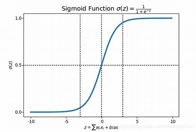
sigmoid函数的导数:
σ
′
(
z
)
=
σ
(
z
)
(
1
−
σ
(
z
)
)
\sigma'\left(z\right)=\sigma\left(z\right)\left(1-\sigma\left(z\right)\right)
σ′(z)=σ(z)(1−σ(z))
二分类逻辑斯谛回归模型是如下的条件概率分布:
P
(
y
=
1
∣
x
)
=
σ
(
w
⋅
x
+
b
)
=
1
1
+
exp
(
−
(
w
⋅
x
+
b
)
)
=
exp
(
w
⋅
x
+
b
)
1
+
exp
(
w
⋅
x
+
b
)
P
(
y
=
0
∣
x
)
=
1
−
σ
(
w
⋅
x
+
b
)
=
1
1
+
exp
(
w
⋅
x
+
b
)
\begin{aligned} P \left( y = 1 | \mathbf{x} \right) &=\sigma\left(\mathbf{w}\cdot\mathbf{x}+b\right) \\ &= \dfrac{1}{1+\exp{\left(-\left(\mathbf{w} \cdot \mathbf{x} + b \right)\right)}} \\ &= \dfrac{\exp{\left(\mathbf{w} \cdot \mathbf{x} + b \right)}}{1+\exp{\left( \mathbf{w} \cdot \mathbf{x} + b \right)}}\\ P \left( y = 0 | \mathbf{x} \right) &= 1- \sigma\left(\mathbf{w}\cdot\mathbf{x}+b\right) \\ &=\dfrac{1}{1+\exp{\left( \mathbf{w} \cdot \mathbf{x} + b \right)}}\end{aligned}
P(y=1∣x)P(y=0∣x)=σ(w⋅x+b)=1+exp(−(w⋅x+b))1=1+exp(w⋅x+b)exp(w⋅x+b)=1−σ(w⋅x+b)=1+exp(w⋅x+b)1
其中,
x
∈
R
n
\mathbf{x} \in \mathbb{R}^{n}
x∈Rn,
y
∈
{
0
,
1
}
y \in \left\{ 0, 1 \right\}
y∈{0,1},
w
∈
R
n
\mathbf{w} \in \mathbb{R}^{n}
w∈Rn是权值向量,
b
∈
R
b \in \mathbb{R}
b∈R是偏置,
w
⋅
x
\mathbf{w} \cdot \mathbf{x}
w⋅x为向量内积。
可将权值权值向量和特征向量加以扩充,即增广权值向量
w
^
=
(
w
(
1
)
,
w
(
2
)
,
⋯
,
w
(
n
)
,
b
)
⊤
\hat{\mathbf{w}} = \left( w^{\left(1\right)},w^{\left(2\right)},\cdots,w^{\left(n\right)},b \right)^\top
w^=(w(1),w(2),⋯,w(n),b)⊤,增广特征向量
x
^
=
(
x
(
1
)
,
x
(
2
)
,
⋯
,
x
(
n
)
,
1
)
⊤
\hat{\mathbf{x}} = \left( x^{\left(1\right)},x^{\left(2\right)},\cdots,x^{\left(n\right)},1 \right)^\top
x^=(x(1),x(2),⋯,x(n),1)⊤,则逻辑斯谛回归模型:
P
(
y
=
1
∣
x
^
)
=
exp
(
w
^
⋅
x
^
)
1
+
exp
(
w
^
⋅
x
^
)
P
(
y
=
0
∣
x
^
)
=
1
1
+
exp
(
w
^
⋅
x
^
)
\begin{aligned} \\& P \left( y = 1 | \hat{\mathbf{x}} \right) = \dfrac{\exp{\left(\hat{\mathbf{w}} \cdot \hat{\mathbf{x}} \right)}}{1+\exp{\left( \hat{\mathbf{w}} \cdot \hat{\mathbf{x}} \right)}}\\& P \left( y = 0 | \hat{\mathbf{x}} \right) =\dfrac{1}{1+\exp{\left( \hat{\mathbf{w}} \cdot \hat{\mathbf{x}} \right)}}\end{aligned}
P(y=1∣x^)=1+exp(w^⋅x^)exp(w^⋅x^)P(y=0∣x^)=1+exp(w^⋅x^)1
2.2 二分类逻辑斯谛回归参数学习——最大似然估计
给定训练数据集
D
=
{
(
x
^
1
,
y
1
)
,
(
x
^
2
,
y
2
)
,
⋯
,
(
x
^
N
,
y
N
)
}
\begin{aligned} \\& D = \left\{ \left( \hat{\mathbf{x}}_{1}, y_{1} \right), \left( \hat{\mathbf{x}}_{2}, y_{2} \right), \cdots, \left( \hat{\mathbf{x}}_{N}, y_{N} \right) \right\} \end{aligned}
D={(x^1,y1),(x^2,y2),⋯,(x^N,yN)}
其中,
x
^
i
∈
R
n
+
1
,
y
i
∈
{
0
,
1
}
,
i
=
1
,
2
,
⋯
,
N
\hat{\mathbf{x}}_{i} \in \mathbb{R}^{n+1}, y_{i} \in \left\{ 0, 1 \right\}, i = 1, 2, \cdots, N
x^i∈Rn+1,yi∈{0,1},i=1,2,⋯,N。
设
P
(
y
=
1
∣
x
^
)
=
σ
(
w
^
⋅
x
^
)
,
P
(
y
=
0
∣
x
^
)
=
1
−
σ
(
w
^
⋅
x
^
)
\begin{aligned} \\& P \left( y =1 | \hat{\mathbf{x}} \right) =\sigma \left( \hat{\mathbf{w}}\cdot\hat{\mathbf{x}} \right) ,\quad P \left( y =0 | \hat{\mathbf{x}} \right) = 1 - \sigma \left( \hat{\mathbf{w}}\cdot\hat{\mathbf{x}} \right) \end{aligned}
P(y=1∣x^)=σ(w^⋅x^),P(y=0∣x^)=1−σ(w^⋅x^)
似然函数
L
(
w
^
)
=
∏
i
=
1
N
P
(
y
i
∣
x
^
i
)
=
∏
i
=
1
N
[
σ
(
w
^
⋅
x
^
i
)
]
y
i
[
1
−
σ
(
w
^
⋅
x
^
i
)
]
1
−
y
i
\begin{aligned} L \left( \hat{\mathbf{w}} \right) &= \prod_{i=1}^N P\left(y_i|\hat{\mathbf{x}}_i\right) \\ &= \prod_{i=1}^{N} \left[ \sigma \left( \hat{\mathbf{w}}\cdot\hat{\mathbf{x}}_{i} \right) \right]^{y_{i}}\left[ 1 - \sigma \left( \hat{\mathbf{w}}\cdot\hat{\mathbf{x}}_{i} \right) \right]^{1 - y_{i}}\end{aligned}
L(w^)=i=1∏NP(yi∣x^i)=i=1∏N[σ(w^⋅x^i)]yi[1−σ(w^⋅x^i)]1−yi
因为似然函数累乘会可能出现下溢的情况,可以转换为对数似然函数(累加)
l
(
w
^
)
=
log
L
(
w
^
)
=
∑
i
=
1
N
[
y
i
log
σ
(
w
^
⋅
x
^
i
)
+
(
1
−
y
i
)
log
(
1
−
σ
(
w
^
⋅
x
^
i
)
)
]
\begin{aligned} \\ l \left( \hat{\mathbf{w}} \right) &= \log L \left( \hat{\mathbf{w}} \right) \\ & = \sum_{i=1}^{N} \left[ y_{i} \log \sigma \left( \hat{\mathbf{w}}\cdot\hat{\mathbf{x}}_{i} \right) + \left( 1 - y_{i} \right) \log \left( 1 - \sigma \left( \hat{\mathbf{w}}\cdot\hat{\mathbf{x}}_{i} \right) \right) \right]\end{aligned}
l(w^)=logL(w^)=i=1∑N[yilogσ(w^⋅x^i)+(1−yi)log(1−σ(w^⋅x^i))]
最大似然估计
w
^
∗
=
arg
max
w
^
l
(
w
^
)
\hat{\mathbf{w}}^*=\mathop{\arg\max}_{\hat{\mathbf{w}}} l\left(\hat{\mathbf{w}}\right)
w^∗=argmaxw^l(w^)
最小负对数损失
w
^
∗
=
arg
min
w
^
−
l
(
w
^
)
\hat{\mathbf{w}}^*=\mathop{\arg\min}_{\hat{\mathbf{w}}}-l\left(\hat{\mathbf{w}}\right)
w^∗=argminw^−l(w^)
令
y
^
i
=
σ
(
w
^
⋅
x
^
i
)
\hat{y}_i=\sigma\left(\hat{\mathbf{w}}\cdot\hat{\mathbf{x}}_i\right)
y^i=σ(w^⋅x^i),则对数似然函数
l
(
w
^
)
l\left(\hat{\mathbf{w}}\right)
l(w^)关于
w
^
\hat{\mathbf{w}}
w^的偏导数
∂
l
(
w
^
)
∂
w
^
=
−
∑
i
=
1
N
(
y
i
y
^
i
(
1
−
y
^
i
)
y
^
i
x
^
i
−
(
1
−
y
i
)
y
^
i
(
1
−
y
^
i
)
1
−
y
^
i
x
^
i
)
=
−
∑
i
=
1
N
(
y
i
(
1
−
y
^
i
)
x
^
i
−
(
1
−
y
i
)
y
^
i
x
^
i
)
=
−
∑
i
=
1
N
x
^
i
(
y
i
−
y
^
i
)
\begin{aligned}\frac{\partial l\left(\hat{\mathbf{w}}\right)}{\partial \hat{\mathbf{w}}} &=-\sum_{i=1}^N\left(y_i\frac{\hat{y}_i\left(1-\hat{y}_i\right)}{\hat{y}_i}\hat{\mathbf{x}}_i-\left(1-y_i\right)\frac{\hat{y}_i\left(1-\hat{y}_i\right)}{1-\hat{y}_i}\hat{\mathbf{x}}_i\right)\\ &=-\sum_{i=1}^N\left(y_i\left(1-\hat{y}_i\right)\hat{\mathbf{x}}_i-\left(1-y_i\right)\hat{y}_i\hat{\mathbf{x}}_i\right) \\ &=-\sum_{i=1}^N\hat{\mathbf{x}}_i\left(y_i-\hat{y}_i\right)\end{aligned}
∂w^∂l(w^)=−i=1∑N(yiy^iy^i(1−y^i)x^i−(1−yi)1−y^iy^i(1−y^i)x^i)=−i=1∑N(yi(1−y^i)x^i−(1−yi)y^ix^i)=−i=1∑Nx^i(yi−y^i)
采用梯度下降法,初始化
w
^
=
0
\hat{\mathbf{w}}=\mathbf{0}
w^=0,进行迭代
w
^
t
+
1
←
w
^
t
+
α
∑
i
=
1
N
x
^
i
(
y
i
−
y
^
i
w
^
t
)
\hat{\mathbf{w}}_{t+1}\gets\hat{\mathbf{w}}_t+\alpha\sum_{i=1}^N\hat{\mathbf{x}}_i\left(y_i-\hat{y}_i^{\hat{\mathbf{w}}_t}\right)
w^t+1←w^t+αi=1∑Nx^i(yi−y^iw^t)
其中,
α
\alpha
α是学习率,
y
^
i
w
^
t
\hat{y}_i^{\hat{\mathbf{w}}_t}
y^iw^t是当参数
w
^
t
\hat{\mathbf{w}}_t
w^t时模型的预测输出。
2.3 逻辑斯谛回归模型应用
from math import exp
import numpy as np
import pandas as pd
import matplotlib.pyplot as plt
%matplotlib inline

from sklearn.datasets import load_iris
from sklearn.model_selection import train_test_split
def create_data():
    iris = load_iris()
    df = pd.DataFrame(iris.data, columns=iris.feature_names)
    df['label'] = iris.target
    df.columns = ['sepal length', 'sepal width', 'petal length', 'petal width', 'label']
    data = np.array(df.iloc[:100, [0,1,-1]])
    return data[:, :2], data[:, -1]
X, y = create_data()
X_train, X_test, y_train, y_test = train_test_split(X, y, test_size=0.3)
class LogisticRegressionClassifier:

    def __init__(self, max_iter=200, learning_rate=0.01):
        self.max_iter = max_iter
        self.learning_rate = learning_rate

    def sigmoid(self, x):
        return 1 / (1 + exp(-x))

    def data_matrix(self, X):
        data_mat = []
        for d in X:
            data_mat.append([1.0, *d])
        return data_mat

    def fit(self, X, y):
        data_mat = self.data_matrix(X)
        self.weights = np.zeros((len(data_mat[0]), 1), dtype=np.float32)

        for iter_ in range(self.max_iter):
            for i in range(len(X)):
                result = self.sigmoid(np.dot(data_mat[i], self.weights))
                error = y[i] - result
                self.weights += self.learning_rate * error * np.transpose([data_mat[i]])
        print('LogisticRegression Model(learning_rate={}, max_iter={})'.
              format(self.learning_rate, self.max_iter))

    def score(self, X_test, y_test):
        right = 0
        X_test = self.data_matrix(X_test)
        for x, y in zip(X_test, y_test):
            result = np.dot(x, self.weights)
            if (result > 0 and y == 1) or (result < 0 and y == 0):
                right += 1
        return right / len(X_test)
lr_clf = LogisticRegressionClassifier()
lr_clf.fit(X_train, y_train)
lr_clf.score(X_test, y_test)
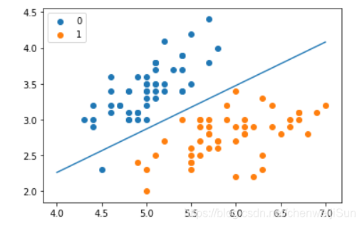
x_points = np.arange(4, 8)
y_ = -(lr_clf.weights[1] * x_points + lr_clf.weights[0]) / lr_clf.weights[2]

plt.plot(x_points, y_)
plt.scatter(X[:50, 0], X[:50, 1], label='0')
plt.scatter(X[50:, 0], X[50:, 1], label='1')
plt.legend()
import matplotlib.pyplot as plt
import numpy as np
from sklearn import datasets, linear_model
from sklearn import model_selection

def load_data():
    iris=datasets.load_iris()
    X_train=iris.data
    y_train=iris.target
    return model_selection.train_test_split(X_train, y_train,test_size=0.25,random_state=0,stratify=y_train)

def test_LogisticRegression(*data):
    X_train,X_test,y_train,y_test=data
    regr = linear_model.LogisticRegression()
    regr.fit(X_train, y_train)
    print('Coefficients:%s, intercept %s'%(regr.coef_,regr.intercept_))
    print('Score: %.2f' % regr.score(X_test, y_test))

def test_LogisticRegression_multinomial(*data):
    X_train,X_test,y_train,y_test=data
    regr = linear_model.LogisticRegression(multi_class='multinomial',solver='lbfgs')
    regr.fit(X_train, y_train)
    print('Coefficients:%s, intercept %s'%(regr.coef_,regr.intercept_))
    print('Score: %.2f' % regr.score(X_test, y_test))

def test_LogisticRegression_C(*data):
    X_train,X_test,y_train,y_test=data
    Cs=np.logspace(-2,4,num=100)
    scores=[]
    for C in Cs:
        regr = linear_model.LogisticRegression(C=C)
        regr.fit(X_train, y_train)
        scores.append(regr.score(X_test, y_test))

    fig=plt.figure()
    ax=fig.add_subplot(1,1,1)
    ax.plot(Cs,scores)
    ax.set_xlabel(r"C")
    ax.set_ylabel(r"score")
    ax.set_xscale('log')
    ax.set_title("LogisticRegression")
    plt.show()

if __name__=='__main__':
    X_train,X_test,y_train,y_test=load_data()
    test_LogisticRegression(X_train,X_test,y_train,y_test)
    test_LogisticRegression_multinomial(X_train,X_test,y_train,y_test)
    test_LogisticRegression_C(X_train,X_test,y_train,y_test)


 1471
1471


 被折叠的 条评论
为什么被折叠?
被折叠的 条评论
为什么被折叠?
 到【灌水乐园】发言


