【Python 机器学习实战】ID3决策树

一、决策树的构造

决策树是一种依托决策而建立起来的一种树。

在机器学习中，决策树是一种预测模型，代表的是一种对象属性与对象值之间的一种映射关系，每一个节点代表某个对象，树中的每一个分叉路径代表某个可能的属性值，而每一个叶子节点则对应从根节点到该叶子节点所经历的路径所表示的对象的值。

• 优点：计算复杂度不高，输出结果易于理解，对中间值的缺失不敏感，可以处理不相关特征数据。
• 缺点：可能会产生过度匹配问题。
• 适用数据类型：数值型和标称型。

决策树的一般流程

（1）收集数据：可以使用任何方法。

（2）准备数据：树构造算法只适用于标称型数据，因此数值型数据必须离散化。

（3）分析数据：可以使用任何方法，构造树完成之后，应检查图形是否符合预期。

（4）训练算法：构造树的数据结构。

（5）测试算法：使用经验树计算错误率。

（6）使用算法：此步骤可以适用于任何监督学习算法，而使用决策树可以更好地理解数据的内在含义。

ID3算法是决策树的一种，它是基于奥卡姆剃刀原理的，即用尽量用较少的东西做更多的事。

ID3算法，即Iterative Dichotomiser 3，迭代二叉树3代，是Ross Quinlan发明的一种决策树算法

1.1 信息增益

在划分数据集之前之后信息发生的变化称为信息增益，获得信息增益最高的特征就是最好的选择。

熵定义为信息的期望值。

如果待分类的事务可能划分在多个分类之中，则符号xi的信息定义为： l(xi) = -log2p(xi), 其中p(xi)是选择该分类的概率。

为了计算熵，需要计算所有类别所有可能值包含的信息期望值，H = -Σ(n,i=1)p(xi)log2p(xi)

计算给定数据集的香农熵

from math import log
import operator
# 内置的操作符函数接口,用 C 实现的，所以执行速度比 Python 代码快。

def calcShannonEnt(dataSet):
    numEntries = len(dataSet)  # 实例总数
    labelCounts = {}  # 所有类标签，字典形式，每个键值都记录了当前类别出现的次数。
    
    # 为所有可能分类创建字典，统计所有类标签发生的次数。
    for featVec in dataSet:
        currentLabel = featVec[-1]  # 类标签
        if currentLabel not in labelCounts.keys():  # 如果当前键值不存在，扩展字典
            labelCounts[currentLabel] = 0
        labelCounts[currentLabel] += 1
        
    # 以2为底求对数
    shannonEnt = 0.0
    for key in labelCounts:
        prob = float(labelCounts[key]) / numEntries  # 使用所有类标签的发生频率计算类别出现的概率
        shannonEnt -= prob * log(prob, 2)
    return shannonEnt
    

# 简单鱼鉴定数据集
def createDataSet():
    dataSet = [[1, 1, 'yes'],
              [1, 1, 'yes'],
              [1, 0, 'no'],
              [0, 1, 'no'],
              [0, 1, 'no']]
    labels = ['no surfacing', 'flippers']  # 不浮出水面、脚蹼
    return dataSet, labels

myDat, labels = createDataSet()
print(myDat)
print(labels)

[[1, 1, 'yes'], [1, 1, 'yes'], [1, 0, 'no'], [0, 1, 'no'], [0, 1, 'no']]
['no surfacing', 'flippers']

calcShannonEnt(myDat)

0.9709505944546686

1.2 划分数据集

按照给定特征划分数据集

# 参数：待划分的数据集、划分数据集的特征、需要返回的特征的值
def splitDataSet(dataSet, axis, value):
    retDataSet = []  # 创建新的list对象
    for featVec in dataSet:
        if featVec[axis] == value:  # 抽取
            reducedFeatVec = featVec[:axis]
            reducedFeatVec.extend(featVec[axis+1:])  # 去除了划分的特征
            retDataSet.append(reducedFeatVec)
    return retDataSet

splitDataSet(myDat, 0, 0)

[[1, 'no'], [1, 'no']]

选择最好的数据集划分方式

def chooseBestFeatureToSplit(dataSet):
    numFeatures = len(dataSet[0]) - 1  # 特征长度，不包括最后一列的类标签
    baseEntropy = calcShannonEnt(dataSet)  # 计算整个数据集的原始香农熵
    bestInfoGain = 0.0; bestFeature = -1  # 最好信息增益，最好特征
    for i in range(numFeatures):
        # 使用列表推导创建新的唯一的分类标签列表，将数据集中所有第i个特征值或者所有可能存在的值写入新list中
        featList = [example[i] for example in dataSet]
        uniqueVals = set(featList)  # 集合类型中的每个值互不相同
        
        # 遍历当前特征中的所有唯一属性值，对每个唯一属性值划分一次数据集，然后计算子数据集的新熵值，并对所有唯一特征值得到的熵求和
        newEntropy = 0.0  # 以第i个特征划分得到的熵
        # 计算每种划分方式的信息熵
        for value in uniqueVals:
            subDataSet = splitDataSet(dataSet, i, value)  # 第i个特征==value
            prob = len(subDataSet) / float(len(dataSet))  # 子集长度和为1
            newEntropy += prob * calcShannonEnt(subDataSet)
        infoGain = baseEntropy - newEntropy
        
        # 计算最好的信息增益
        if (infoGain > bestInfoGain):
            bestInfoGain = infoGain
            bestFeature = i  # 返回最好特征下标
    return bestFeature

数据集需满足：

• 数据必须是一种由列表元素组成的列表，而且所有的列表元素都要具有相同的数据长度；
• 数据的最后一列或者每个实例的最后一个元素是当前实例的类别标签。

chooseBestFeatureToSplit(myDat)

0

1.3 递归构建决策树

如果数据集已经处理了所有属性，但是类标签依然不是唯一的，此时需要决定如何定义该叶子节点，通常采用多数表决的方法决定该叶子节点的分类。

def majorityCnt(classList):
    classCount = {}  # 字典存储了classList中每个类标签出现的频率
    for vote in classList:
        if vote not in classCount.keys():
            classCount[vote] = 0
        classCount[vote] += 1
    sortedClassCount = sorted(classCount.items(), key=operator.itemgetter(1), reverse=True)
    # 排序，返回出现次数最多的分类名称
    # items返回元组字典  输出eg：[('a', 2), ('b', 1), ('c', 1), ('d', 1)]
    return sortedClassCount[0][0]

创建树的函数代码

def createTree(dataSet,labels):
    classList = [example[-1] for example in dataSet]  # 数据集的所有类标签
    # 类别完全相同则停止继续划分，直接返回该类标签
    if classList.count(classList[0]) == len(classList):
        # count()：统计某个元素在列表中出现的次数
        return classList[0]
    # 遍历完所有特征时返回出现次数最多的类别
    if len(dataSet[0]) == 1: # 即：只剩下类标签
        return majorityCnt(classList)
    bestFeat = chooseBestFeatureToSplit(dataSet)  # 最好特征下标
    bestFeatLabel = labels[bestFeat]  # 最好特征标签
    myTree = {bestFeatLabel:{}}
    del(labels[bestFeat])  # 从标签列表里删除已选择标签
    # 得到列表包含的所有最好特征值
    featValues = [example[bestFeat] for example in dataSet]
    uniqueVals = set(featValues)  # 去重，唯一
    for value in uniqueVals:
        subLabels = labels[:]  # 子标签中已经不包括选择过的最好特征标签
        myTree[bestFeatLabel][value] = createTree(splitDataSet(dataSet, bestFeat, value), subLabels)
    return myTree

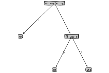
myTree = createTree(myDat, labels)
print(myTree)

{'no surfacing': {0: 'no', 1: {'flippers': {0: 'no', 1: 'yes'}}}}

二、在Python中使用Matplotlib注解绘制树形图

2.1 Matplotlib注解

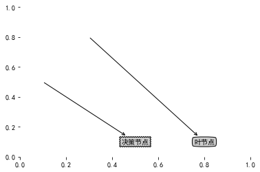
使用文本注解绘制树节点

matplotlib命令与格式：标题(title),标注(annotate),文字说明(text)：https://blog.csdn.net/helunqu2017/article/details/78659490/

import matplotlib.pyplot as plt
# 显示中文
from pylab import *
mpl.rcParams['font.sans-serif'] = ['SimHei']

# 定义文本框和箭头格式
# 定义决策树决策结果的属性，用字典来定义  
# 下面的字典定义也可写作 decisionNode={boxstyle:'sawtooth',fc:'0.8'}  
# boxstyle为文本框的类型，sawtooth是锯齿形，fc是背景颜色深浅
decisionNode = dict(boxstyle="sawtooth", fc="0.8")
leafNode = dict(boxstyle="round4", fc="0.8")
arrow_args = dict(arrowstyle="<-")  # 箭头样式

# 绘制带箭头的注解
# 节点文本，centerPt节点中心坐标  parentPt 起点坐标  节点类型
def plotNode(nodeTxt, centerPt, parentPt, nodeType):
    # annotations注解工具，可以在数据图形上添加文本工具
    # xy 为被注释的坐标点
    # xytext 为注释文字的坐标位置
    # axes fraction 左下角部分
    # bbox给标题增加外框
    createPlot.ax1.annotate(nodeTxt, xy=parentPt, xycoords='axes fraction', xytext=centerPt, textcoords='axes fraction',\
                           va="center", ha="center", bbox=nodeType, arrowprops=arrow_args)
    
def createPlot():
    fig = plt.figure(1, facecolor='white')  # 定义一个画布，背景为白色
    fig.clf()  # 清空绘图区
    # createPlot.ax1为全局变量，绘制图像的句柄，subplot为定义了一个绘图，111表示figure中的图有1行1列，即1个，最后的1代表第一个图 
    # frameon表示是否绘制坐标轴矩形
    createPlot.ax1 = plt.subplot(111, frameon=False)
    plotNode('决策节点', (0.5, 0.1), (0.1, 0.5), decisionNode)
    plotNode('叶节点', (0.8, 0.1), (0.3, 0.8), leafNode)
    plt.show()

createPlot()

2.2 构造注解树

多少个叶节点——可以正确确定x轴的程度；

树有多少层——可以正确确定y轴的高度。

获取叶节点的数目和树的层数

def getNumLeafs(myTree):
    numLeafs = 0
    firstStr = list(myTree.keys())[0]  # 第一个关键字是第一次划分数据集的类别标签
    secondDict = myTree[firstStr]  # 附带的数值表示子节点的取值
    for key in list(secondDict.keys()):
        # 测试节点的数据类型是否为字典，如果子节点是字典类型，则该节点也是一个判断节点
        if type(secondDict[key]).__name__=='dict':
            numLeafs += getNumLeafs(secondDict[key])
        else: numLeafs += 1
    return numLeafs

def getTreeDepth(myTree):
    maxDepth = 0
    firstStr = list(myTree.keys())[0]
    secondDict = myTree[firstStr]
    for key in list(secondDict.keys()):
        # 计算遍历过程中遇到判断节点的个数，终止条件为叶子节点
        if type(secondDict[key]).__name__=='dict':
            thisDepth = 1 + getTreeDepth(secondDict[key])
        else: thisDepth = 1
        if thisDepth > maxDepth: 
            maxDepth = thisDepth
    return maxDepth

# 用于测试
def retrieveTree(i):
    listOfTrees = [{'no surfacing': {0: 'no', 1: {'flippers': \
                    {0: 'no', 1: 'yes'}}}},
                   {'no surfacing': {0: 'no', 1: {'flippers': \
                     {0: {'head': {0: 'no', 1: 'yes'}}, 1: 'no'}}}}
                  ]
    return listOfTrees[i]

print(retrieveTree(1))
print(list(retrieveTree(1).keys()))

{'no surfacing': {0: 'no', 1: {'flippers': {0: {'head': {0: 'no', 1: 'yes'}}, 1: 'no'}}}}
['no surfacing']

myTree = retrieveTree(0)
print(getNumLeafs(myTree))
print(getTreeDepth(myTree))

3
2

plotTree函数

def plotMidText(cntrPt, parentPt, txtString):
    # 在父子节点间填充文本信息
    xMid = (parentPt[0]-cntrPt[0])/2.0 + cntrPt[0]
    yMid = (parentPt[1]-cntrPt[1])/2.0 + cntrPt[1]
    createPlot.ax1.text(xMid, yMid, txtString)
    
def plotTree(myTree, parentPt, nodeTxt):
    # 起点坐标为（0.5,1.0）
    # 计算宽与高
    numLeafs = getNumLeafs(myTree)
    depth = getTreeDepth(myTree)
    
    firstStr = list(myTree.keys())[0]  # 第一个判断节点
    # (叶子节点数+1) * 半叶距  
    cntrPt = (plotTree.xOff + (1.0 + float(numLeafs))/2.0/plotTree.totalW, plotTree.yOff)
    # 标记子节点属性值
    plotMidText(cntrPt, parentPt, nodeTxt)
    plotNode(firstStr, cntrPt, parentPt, decisionNode)
    secondDict = myTree[firstStr]
    # 减少y偏移
    plotTree.yOff = plotTree.yOff - 1.0/plotTree.totalD
    for key in list(secondDict.keys()):
        if type(secondDict[key]).__name__=='dict':
            plotTree(secondDict[key], cntrPt, str(key))
        else:
            plotTree.xOff = plotTree.xOff + 1.0/plotTree.totalW
            plotNode(secondDict[key], (plotTree.xOff, plotTree.yOff), cntrPt, leafNode)
            plotMidText((plotTree.xOff, plotTree.yOff), cntrPt, str(key))
    # yOff在进入下一层时要减一个层距，跳出时要加回来
    plotTree.yOff = plotTree.yOff + 1.0/plotTree.totalD
    
# 绘制图形是按照比例绘制树形图，好处是无需关心实际输出的图形大小
# x轴和y轴的有效范围是0.0-1.0
def createPlot(inTree):
    fig = plt.figure(1, facecolor='white')
    fig.clf()
    axprops = dict(xticks=[], yticks=[])  # x,y轴值设为空
    createPlot.ax1 = plt.subplot(111, frameon=False, **axprops)
    # 使用这两个变量可以计算树的节点的摆放位置，这样可以将树绘制在水平方向和垂直方向的中心位置
    plotTree.totalW = float(getNumLeafs(inTree))  # 全局变量
    plotTree.totalD = float(getTreeDepth(inTree))
    # 追踪已经绘制的节点位置，以及放置下一个节点的恰当位置
    # plotTree.xOff的值  只有真的画了一个叶节点，才改变xOff的值
    plotTree.xOff = -0.5/plotTree.totalW; plotTree.yOff = 1.0;  
    # 将1/plotTree.totalW称为"叶距"，即叶子节点数等分划分x轴后的每一段大小，称二分之一个"叶距"为"半叶距"。
    # 决策树的最左边的叶节点距离图的左边界相隔一个"半叶距", 最右边的叶节点距离图的右边界相隔一个"半叶距"
    # 初始的xOff与第一个叶节点也要相差一个“叶距”，所以xOff相对y轴左移了一个“半叶距”
    plotTree(inTree, (0.5,1.0), '')
    plt.show()

myTree = retrieveTree(0)
createPlot(myTree)

三、测试和存储分类器

3.1 测试算法：使用决策树执行分类

使用决策树的分类函数

def classify(inputTree, featLabels, testVec):
    firstStr = list(inputTree.keys())[0]
    secondDict = inputTree[firstStr]
    # 将标签字符串转换为索引
    featIndex = featLabels.index(firstStr)  # 查找标签列表中第一个匹配firstStr变量的索引
    for key in list(secondDict.keys()):
        if testVec[featIndex] == key:  # 待测试数据 标签值 == 决策树中线上值
            if type(secondDict[key]).__name__=='dict':
                classLabel = classify(secondDict[key], featLabels, testVec)
            else:
                classLabel = secondDict[key]
    return classLabel

myDat, labels = createDataSet()
print(labels)
myTree = retrieveTree(0)
print(myTree)
print(classify(myTree, labels, [1,0]))
print(classify(myTree, labels, [1,1]))

['no surfacing', 'flippers']
{'no surfacing': {0: 'no', 1: {'flippers': {0: 'no', 1: 'yes'}}}}
no
yes

3.2 使用算法：决策树的存储

使用pickle模块序列化对象存储决策树

def storeTree(inputTree, filename):
    import pickle
    fw = open(filename, 'wb')
    pickle.dump(inputTree,fw)  # 使用dump()将数据序列化到文件中
    fw.close()
    
def grabTree(filename):
    import pickle
    fr = open(filename, 'rb') 
    # 使用load()将数据从文件中序列化读出 
    return pickle.load(fr)

storeTree(myTree, '../datasets/lenses/classifierStorage.txt')
grabTree('../datasets/lenses/classifierStorage.txt')

{'no surfacing': {0: 'no', 1: {'flippers': {0: 'no', 1: 'yes'}}}}

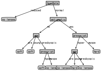
四、使用决策树预测隐形眼镜类型

隐形眼镜数据集，它包含很多患者眼部状况的观察条件以及医生推荐的隐形眼镜类型。

隐形眼镜类型包括硬材质、软材质以及不适合佩戴隐形眼镜。

fr = open('../datasets/lenses/lenses.txt')
lenses = [inst.strip().split('\t') for inst in fr.readlines()]
lensesLabels = ['age', 'prescript', 'astigmatic', 'tearRate']
lensesTree = createTree(lenses, lensesLabels)
print(lensesTree)
createPlot(lensesTree)

{'tearRate': {'reduced': 'no lenses', 'normal': {'astigmatic': {'no': {'age': {'pre': 'soft', 'young': 'soft', 'presbyopic': {'prescript': {'hyper': 'soft', 'myope': 'no lenses'}}}}, 'yes': {'prescript': {'hyper': {'age': {'pre': 'no lenses', 'young': 'hard', 'presbyopic': 'no lenses'}}, 'myope': 'hard'}}}}}}

ID3算法无法直接处理数值型数据。

隐形眼镜的例子表明决策树可能会产生过多的数据集划分，从而产生过度匹配数据集的问题。我们可以通过裁减决策树，合并相邻的无法产生大量信息增益的叶节点，消除过度匹配问题。

转载于:https://my.oschina.net/u/4004713/blog/3017180