python3d画图mpl_toolkits.mplot3d

Line plot

# -*- coding: utf-8 -*-
import numpy as np
import matplotlib as mpl
import matplotlib.pyplot as plt
from mpl_toolkits.mplot3d import Axes3D

mpl.rcParams['legend.fontsize'] = 20  # mpl模块载入的时候加载配置信息存储在rcParams变量中，rc_params_from_file()函数从文件加载配置信息

font = {
    'color': 'b',
    'style': 'oblique',
    'size': 20,
    'weight': 'bold'
}
fig = plt.figure(figsize=(16, 12))  #参数为图片大小
ax = fig.gca(projection='3d')  # get current axes，且坐标轴是3d的

# 准备数据
theta = np.linspace(-8 * np.pi, 8 * np.pi, 100)  # 生成等差数列，[-8π,8π]，个数为100
z = np.linspace(-2, 2, 100)  # [-2,2]容量为100的等差数列，这里的数量必须与theta保持一致，因为下面要做对应元素的运算
r = z ** 2 + 1
x = r * np.sin(theta)  # [-5,5]
y = r * np.cos(theta)  # [-5,5]
ax.set_xlabel("X", fontdict=font)
ax.set_ylabel("Y", fontdict=font)
ax.set_zlabel("Z", fontdict=font)
ax.set_title("Line Plot", alpha=0.5, fontdict=font) #alpha参数指透明度transparent
ax.plot(x, y, z, label='parametric curve')
ax.legend(loc='upper right') #legend的位置可选：upper right/left/center,lower right/left/center,right,left,center,best等等

plt.show()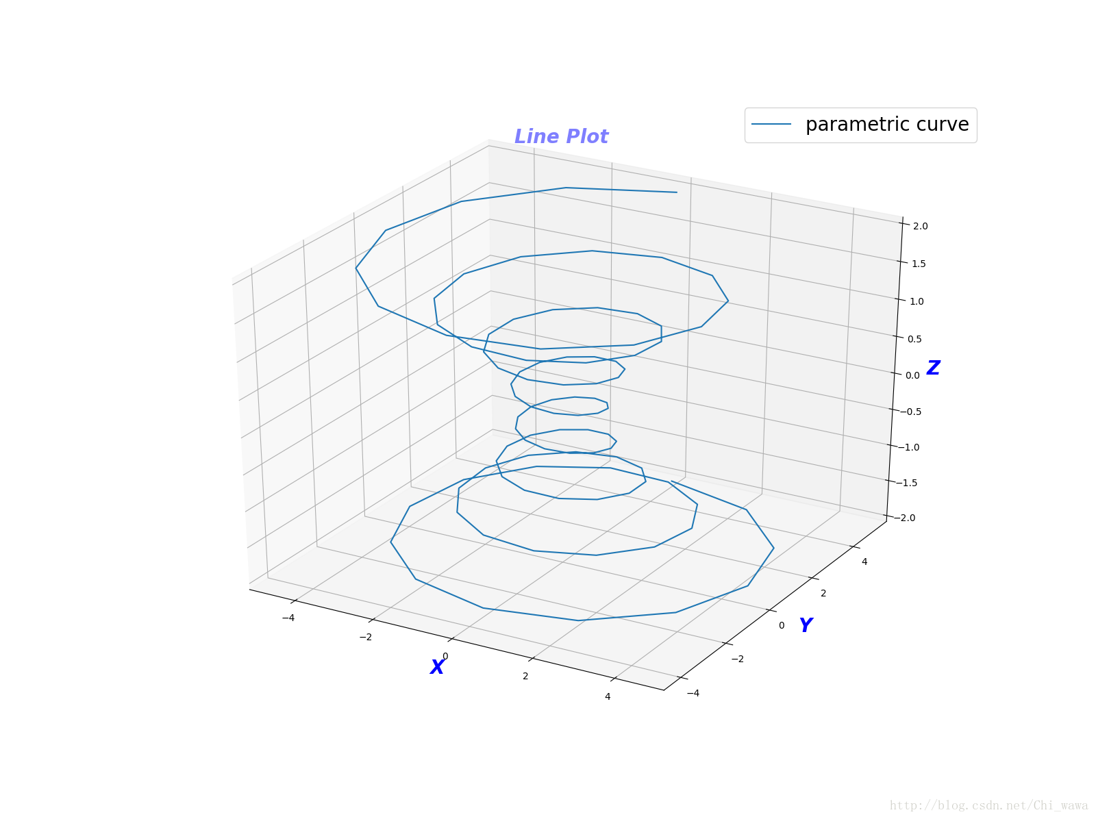

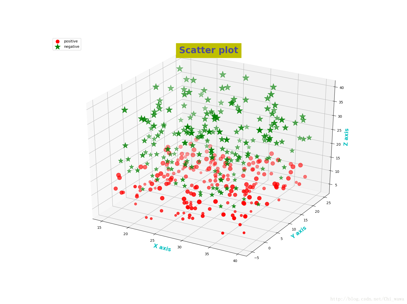
Scatter plot

# -*- coding: utf-8 -*-
import numpy as np
import matplotlib as mpl
import matplotlib.pyplot as plt
from mpl_toolkits.mplot3d import Axes3D

label_font = {
    'color': 'c',
    'size': 15,
    'weight': 'bold'
}


def randrange(n, vmin, vmax):
    r = np.random.rand(n)  # 随机生成n个介于0~1之间的数
    return (vmax - vmin) * r + vmin  # 得到n个[vmin,vmax]之间的随机数


fig = plt.figure(figsize=(16, 12))
ax = fig.add_subplot(111, projection="3d")  # 添加子坐标轴，111表示1行1列的第一个子图
n = 200
for zlow, zhigh, c, m, l in [(4, 15, 'r', 'o', 'positive'),
                             (13, 40, 'g', '*', 'negative')]:  # 用两个tuple，是为了将形状和颜色区别开来
    x = randrange(n, 15, 40)
    y = randrange(n, -5, 25)
    z = randrange(n, zlow, zhigh)
    ax.scatter(x, y, z, c=c, marker=m, label=l, s=z * 10) #这里marker的尺寸和z的大小成正比

ax.set_xlabel("X axis", fontdict=label_font)
ax.set_ylabel("Y axis", fontdict=label_font)
ax.set_zlabel("Z axis", fontdict=label_font)
ax.set_title("Scatter plot", alpha=0.6, color="b", size=25, weight='bold', backgroundcolor="y")   #子图的title
ax.legend(loc="upper left")    #legend的位置左上

plt.show()

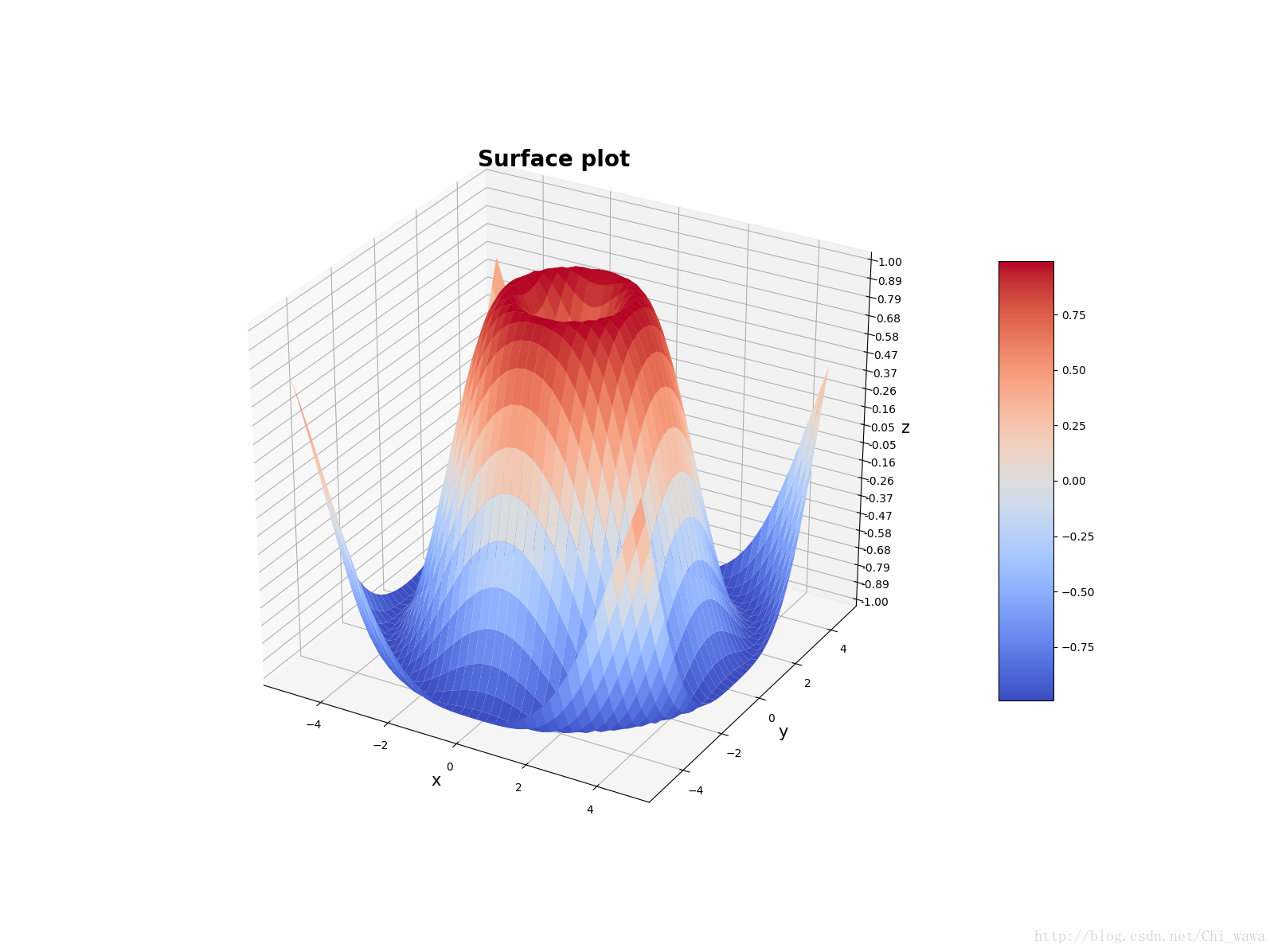
Surface plot

# -*- coding: utf-8 -*-
import numpy as np
import matplotlib.pyplot as plt
from mpl_toolkits.mplot3d import Axes3D
from matplotlib import cm
from matplotlib.ticker import LinearLocator, FormatStrFormatter

fig = plt.figure(figsize=(16,12))
ax = fig.gca(projection="3d")

# 准备数据
x = np.arange(-5, 5, 0.25)    #生成[-5,5]间隔0.25的数列，间隔越小，曲面越平滑
y = np.arange(-5, 5, 0.25)
x, y = np.meshgrid(x,y)  #格点矩阵,原来的x行向量向下复制len(y)次，形成len(y)*len(x)的矩阵，即为新的x矩阵；原来的y列向量向右复制len(x)次，形成len(y)*len(x)的矩阵，即为新的y矩阵；新的x矩阵和新的y矩阵shape相同
r = np.sqrt(x ** 2 + y ** 2)
z = np.sin(r)

surf = ax.plot_surface(x, y, z, cmap=cm.coolwarm)  # cmap指color map

# 自定义z轴
ax.set_zlim(-1, 1)
ax.zaxis.set_major_locator(LinearLocator(20))  # z轴网格线的疏密，刻度的疏密，20表示刻度的个数
ax.zaxis.set_major_formatter(FormatStrFormatter('%.02f'))  # 将z的value字符串转为float，保留2位小数

#设置坐标轴的label和标题
ax.set_xlabel('x',size=15)
ax.set_ylabel('y',size=15)
ax.set_zlabel('z',size=15)
ax.set_title("Surface plot", weight='bold', size=20)

#添加右侧的色卡条
fig.colorbar(surf, shrink=0.6, aspect=8)  # shrink表示整体收缩比例，aspect仅对bar的宽度有影响，aspect值越大，bar越窄
plt.show()

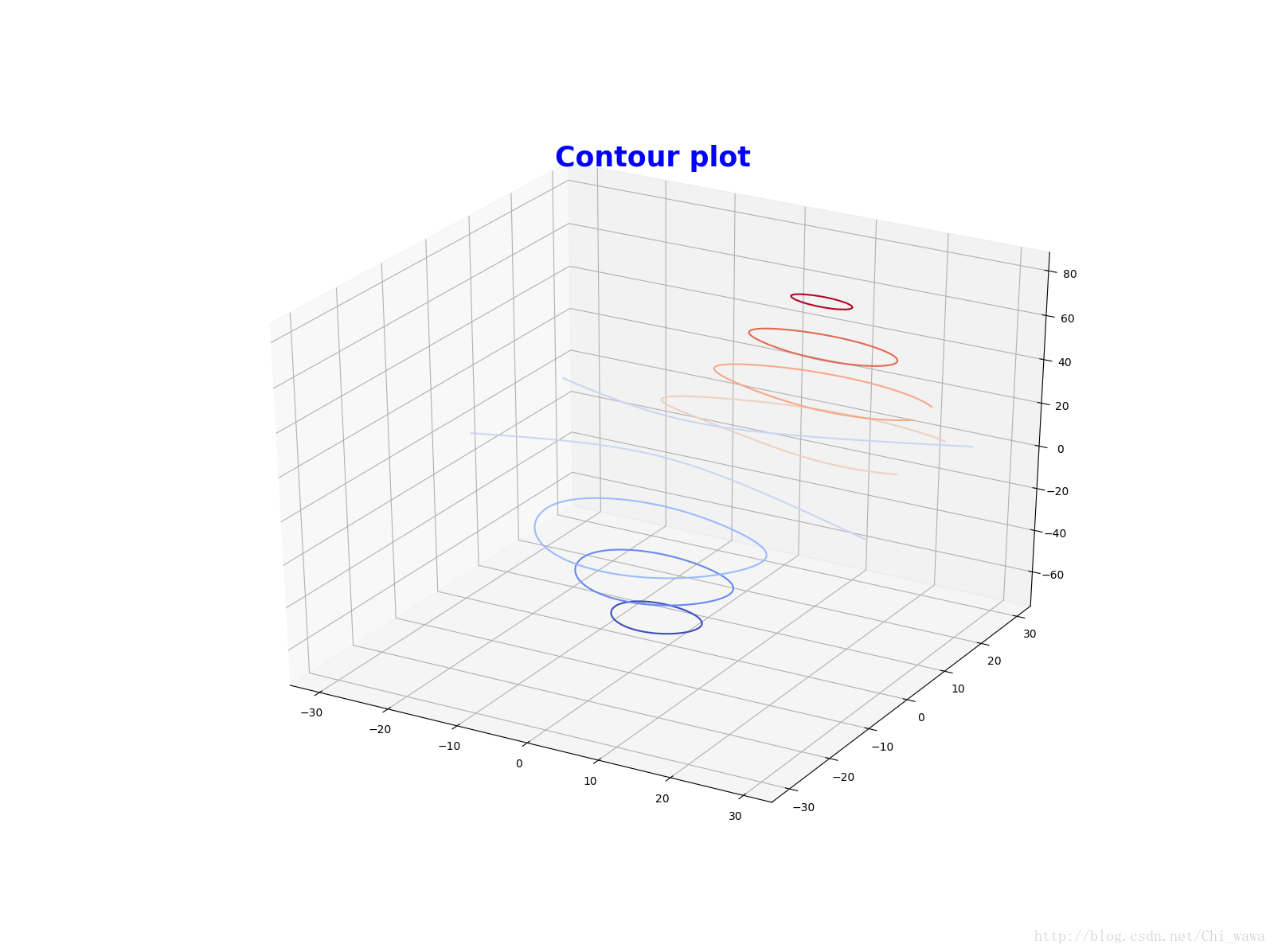
Contour plot

# -*- coding: utf-8 -*-
from mpl_toolkits.mplot3d import axes3d
import matplotlib.pyplot as plt
from matplotlib import cm

fig = plt.figure(figsize=(16, 12))
ax = fig.add_subplot(111, projection='3d')
X, Y, Z = axes3d.get_test_data(0.05)       #测试数据
cset = ax.contour(X, Y, Z, cmap=cm.coolwarm)  #color map选用的是coolwarm
#cset = ax.contour(X, Y, Z,extend3d=True, cmap=cm.coolwarm)
ax.set_title("Contour plot", color='b', weight='bold', size=25)
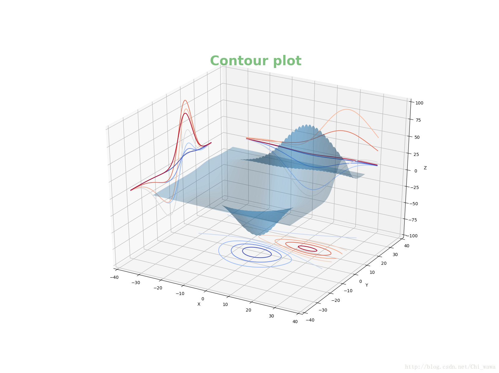
plt.show()

以下两图分别是未设置extend3d属性和设置extend3d属性为True的轮廓图：

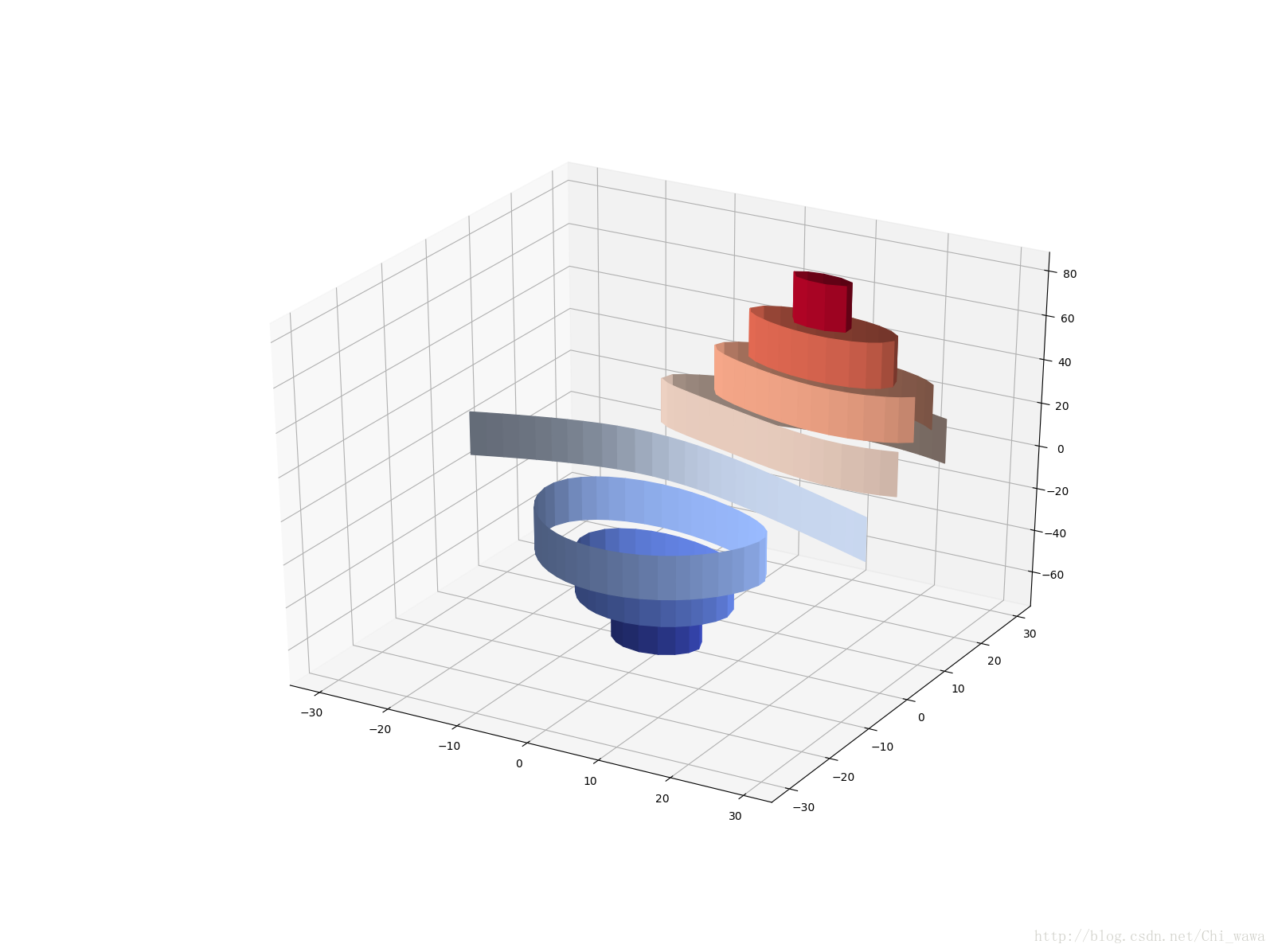
# -*- coding: utf-8 -*-
import numpy as np
import matplotlib.pyplot as plt
from matplotlib import cm
from mpl_toolkits.mplot3d import axes3d

fig = plt.figure(figsize=(16, 12))
ax = fig.gca(projection="3d")  # get current axis
X, Y, Z = axes3d.get_test_data(0.05)  #测试数据

ax.plot_surface(X, Y, Z, rstride=3, cstride=3, alpha=0.3)
cset = ax.contour(X, Y, Z, zdir='z', offset=-100, cmap=cm.coolwarm)
cset = ax.contour(X, Y, Z, zdir="x", offset=-40, cmap=cm.coolwarm)
cset = ax.contour(X, Y, Z, zdir="y", offset=40, cmap=cm.coolwarm)

ax.set_xlabel('X')
ax.set_xlim(-40, 40)
ax.set_ylabel('Y')
ax.set_ylim(-40, 40)
ax.set_zlabel('Z')
ax.set_zlim(-100, 100)
ax.set_title('Contour plot', alpha=0.5, color='g', weight='bold', size=30)

plt.show()

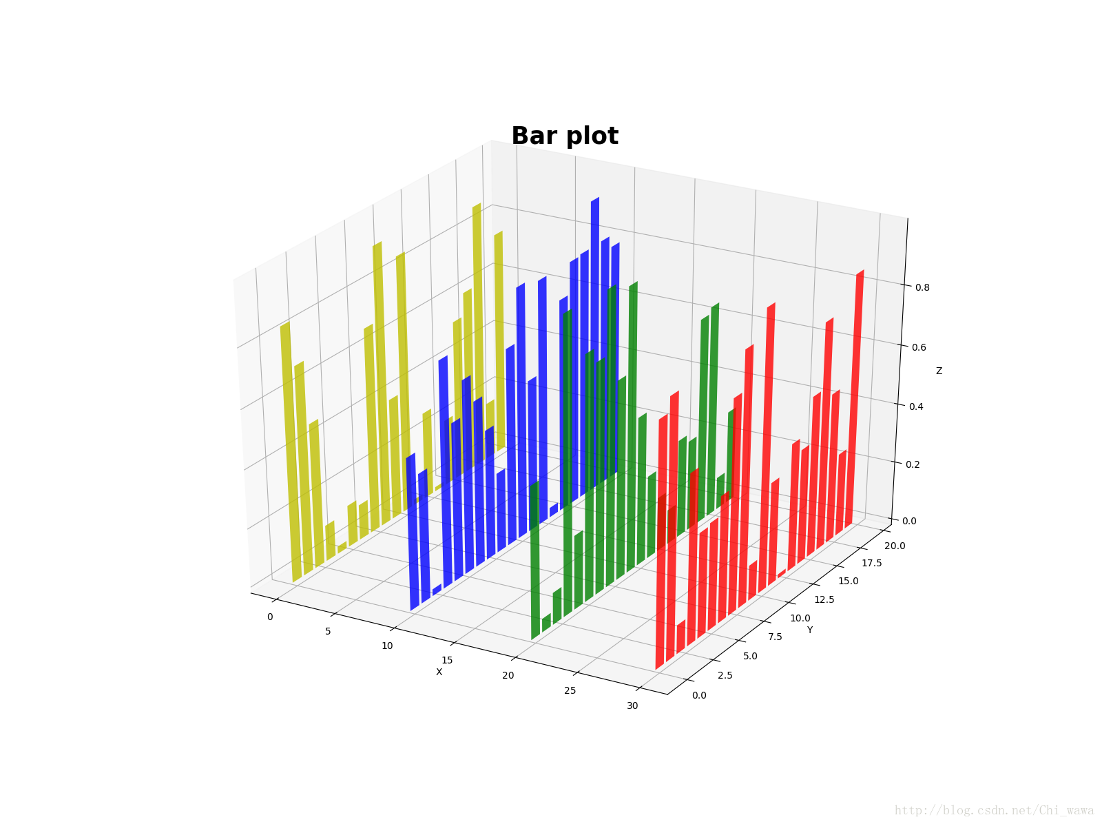
Bar plot

# -*- coding: utf-8 -*-
import numpy as np
import matplotlib.pyplot as plt
from mpl_toolkits.mplot3d import Axes3D

fig = plt.figure(figsize=(16, 12))
ax = fig.add_subplot(111, projection="3d")
a = zip(['r', 'g', 'b', 'y'], [30, 20, 10, 0])
for c, z in a:
    xs = np.arange(20)  # [0,20)之间的自然数,共20个
    ys = np.random.rand(20)  # 生成20个[0,1]之间的随机数
    cs = [c] * len(xs)  # 生成颜色列表
    ax.bar(xs, ys, z, zdir='x', color=cs, alpha=0.8)  # 以zdir='x'，指定z的方向为x轴，那么x轴取值为[30,20,10,0]
#   ax.bar(xs, ys, z, zdir='y', color=cs, alpha=0.8)
#   ax.bar(xs, ys, z, zdir='z', color=cs, alpha=0.8)

ax.set_xlabel('X')
ax.set_ylabel('Y')
ax.set_zlabel('Z')
ax.set_title('Bar plot', size=25, weight='bold')
plt.show()

2D plot in 3D

# -*- coding: utf-8 -*-
import numpy as np
import matplotlib.pyplot as plt
from mpl_toolkits.mplot3d import Axes3D

fig = plt.figure(figsize=(16, 12))
ax = fig.gca(projection="3d")

# 在x轴和y轴画sin函数
x = np.linspace(0, 1, 100)
y = np.sin(2 * np.pi * x) + 1  # 2*π*x∈[0,2π] y属于[0,2]
ax.plot(x, y, zs=0, zdir='z', label="sin curve in (x,y)")

colors = ('r', 'g', 'b', 'k')
x = np.random.sample(20 * len(colors))
y = np.random.sample(20 * len(colors))
c_list = []
for c in colors:
    c_list.append([c] * 20)  # 比如，[colors[0]*5]的结果是['r','r','r','r','r']，是个list
ax.scatter(x, y, zs=0, zdir='y', c=c_list, label="scatter points in (x,z)")

ax.legend()
ax.set_xlim(0, 1)
ax.set_ylim(0, 2)
ax.set_zlim(0, 1)
ax.set_xlabel("X")
ax.set_ylabel("Y")
ax.set_zlabel("Z")

ax.view_init(elev=20, azim=25)  # 调整坐标轴的显示角度
plt.show()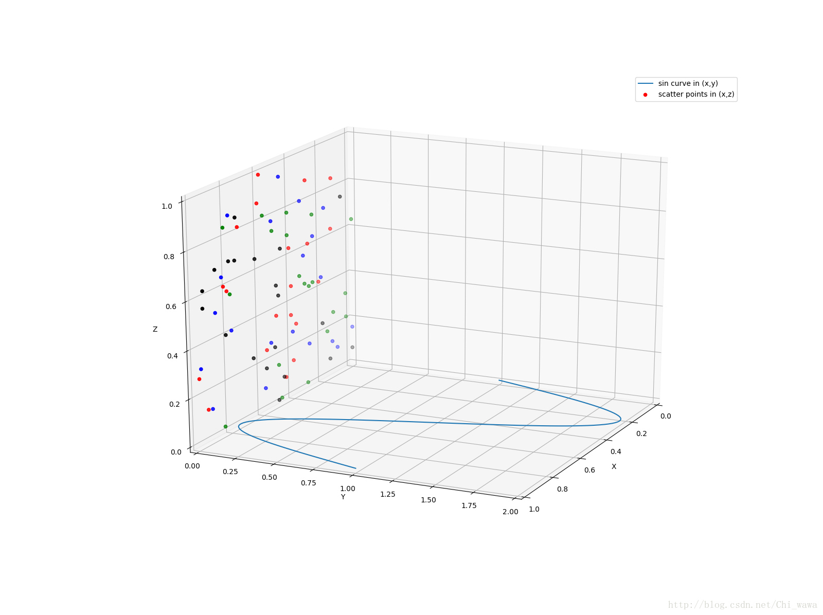

Subplot

# -*- coding: utf-8 -*-
import numpy as np
import matplotlib.pyplot as plt
from matplotlib import cm
from mpl_toolkits.mplot3d import axes3d
from matplotlib.ticker import LinearLocator, FormatStrFormatter

fig = plt.figure(figsize=plt.figaspect(0.5))  # figure的高度是宽度的0.5倍

# 子图1
ax = fig.add_subplot(121, projection="3d")
X = np.arange(-5, 5, 0.25)  # 生成的List的间隔为0.25
Y = np.arange(-5, 5, 0.25)
X, Y = np.meshgrid(X, Y)
R = np.sqrt(X ** 2 + Y ** 2)
Z = np.sin(R)

surf = ax.plot_surface(X, Y, Z, cmap=cm.coolwarm)
ax.set_zlim(-2, 2)
ax.zaxis.set_major_locator(LinearLocator(20))
ax.zaxis.set_major_formatter(FormatStrFormatter('%.02f'))
fig.colorbar(surf, shrink=0.6, aspect=10)

# 子图2
ax = fig.add_subplot(122, projection="3d")
X, Y, Z = axes3d.get_test_data(0.05)
ax.plot_wireframe(X, Y, Z)
plt.show()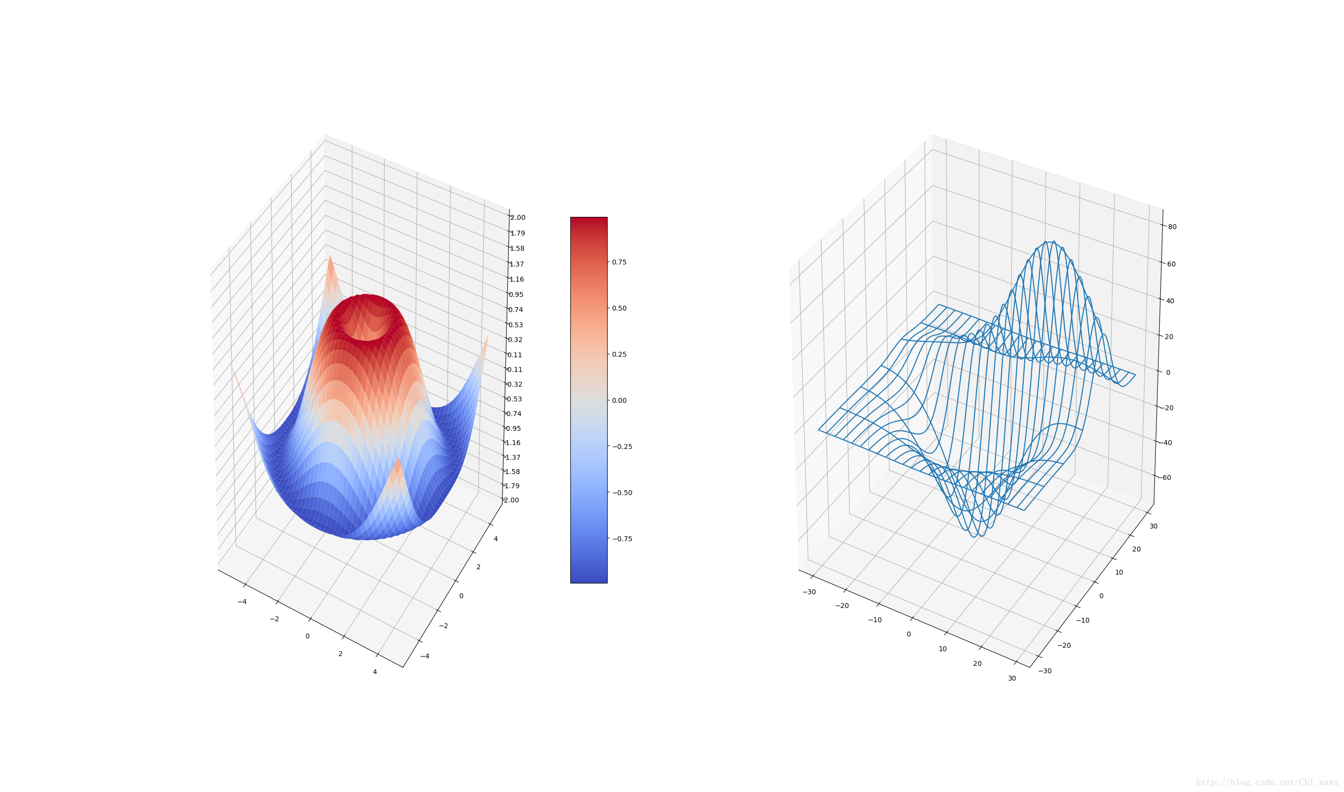

参考文献：mplot3d官方文档
mplot3d官方API