常用损失函数及tf实现

置顶 yichudu

已于 2024-03-22 11:26:07 修改

阅读量1.7k

点赞数 2

分类专栏：【ML------------通用文章标签：深度学习

于 2019-05-07 14:32:28 首次发布

天天开心

本文链接：https://blog.csdn.net/chuchus/article/details/89920480

版权

【ML------------通用专栏收录该内容

32 篇文章 1 订阅

订阅专栏

一. Cross Entropy 交叉熵

交叉熵可以用来衡量两个概率分布之间的差异, 熵越小表明差异越小, 故可用作损失函数.

预备知识: KL 散度

KL散度, Kullback-Leibler divergence, 由名字中的两人在1951年提出,
是两个概率分布 P 和 Q 之间的一个非对称的度量公式.
离散空间下, 从Q到P的KL散度为

$\begin{aligned} D_{KL}(P||Q) &= \sum_i P(i) log\frac{P(i)}{Q(i)} \\ & = \sum_i P(i) log {P(i)}-\sum_i P(i) log{Q(i)} \end{aligned}$
因为非对称, 所以 $D_{KL}(P||Q) \ne D_{KL}(Q||P)$
相应的,连续空间下两个概率密度函数 p,q , 从Q到P的KL散度为:
$D_{KL}(p||q)=\int_X p(x) log\frac{p(x)}{q(x)}\mathrm dx$
习惯用P表示理论分布, Q表示真实分布, $D_{KL}(Q||P)$ 就表示真实分布与理想分布间的差距.

交叉熵表达式

交叉熵与KL散度的关系为: A和B的交叉熵 = A与B的KL散度 - A的熵

二分类中, 可以表示为式(3).
$\ln \hat y + (1-y ) \ln (1-\hat y)] \tag 3$
where $\in \{0,1\}$ , $\hat y \in [0,1] {}$ , $\hat y$ 由 logistic 或 softmax得到.
它也叫 binary_cross_entropy, log_loss.
使用场景: RecSys ctr预估中的正(点击)负(曝光未点击)样本分类.
引申讨论
Q: 当loss下降时, 模型的 metric 一定会提升么?
A: 不总是这样. 当一个数据集的ctr=0.05时, 输出恒为p=0.05时, 此时loss为0.198, 而auc是0.5 .
```
import numpy as np
p = 0.05
ce = -(p * np.log(p) + (1 - p) * np.log(1 - p))  # 结果为 0.198
```
多分类
是指多类别, 一个 sample 只能归属到一个确定的类别.
$L=\sum_{i=1}^{类别数n}-(y_i \ln \hat y_i ) \tag {4}$

在这里插入图片描述

超大规模分类

有些分类任务中的类别数会很大, 如NLP任务中的词典大小达百万级别, 又如推荐系统中的召回任务,推荐池大小可达千万量级.
此时, 为了得到 loss,需要

计算网络中某一层输出在所有类别上的logits
对这些 logits 进行 soft_max 计算, 内部又涉及复杂度高的指数运算

以上两步的计算代价在类别数达百万级时会非常耗时, 大大降低训练效率甚至内存溢出难以训练. 通常会用采样的方法控制 logits 及 loss 计算时涉及到的类别数.
此时, 涉及的类别数不再是整个词典大小, 而是K个(超参, 例如取值为100), 由样本所属的正类别和采样(按照热度作 log_unicorm 采样等)得到的负类别构成. 得到 logits后, 如何计算 loss, 又有如下两种方法.

sampled_softmax

对 logits 作 soft_max等后续处理.

NCE

Noise Contrastive Estimation. 对 logits作 sigmoid处理, 这种正规化方式, 不再限制其和为1, 相当于对每种类别作{0,1}二分类.

candidate size 讨论

通常 candidate_size = true_class_num +sampled_calss_num 。
sampled_calss_num 越大，越逼近于 full softmax，理论上对模型性能更友好。

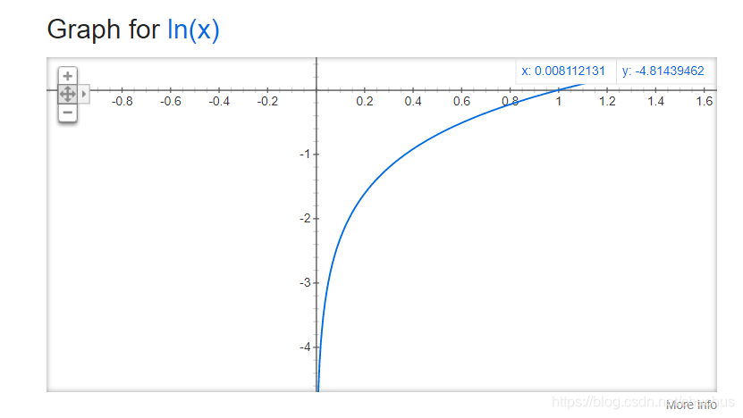
sampled_calss_num 越大，初始训练loss会越高
初始时等价于随机猜，结合交叉熵公式，loss = ln(1/candidate_size). 这里给两个具体值， $l n (1/200) = - 5.29$ , $l n (1/10000) = - 9.21$ .

label smooth 讨论

亲测，若不使用 label_smooth 机制，正负样本比1：199时单机尚能训练，但分布式会 nan loss。继续加大负样本个数则单机、分布式均会 nan loss。
针对以上困扰，加入 label_smooth 机制即可得解。

多标签分类

有多个类别, 一个样本可同时归属于其中的若干个类别. 此时不应再限制logits为一个和为1的概率分布, 类别之间的判断相对独立, 建议用 sigmoid 替代 soft_max. 同理大规模场景下适用NCE.

tf实现

softmax_cross_entropy

tf.losses.softmax_cross_entropy(onehot_labels,logits ,...)
- onehot_labels: [batch_size, num_classes] target one-hot-encoded labels.
- logits: [batch_size, num_classes] logits outputs of the network .
A common use case is to have logits and labels of shape [batch_size, num_classes], but higher dimensions are supported.
labels可以不是one-hot而是一个valid probability distribution, 因为 While the classes are mutually exclusive, their probabilities need not be.

log_softmax

tf.nn.log_softmax(logits, dim=-1, name=None)
数学上等价于先soft_max, 再取log.
意义.
1. 相较于两个api分别先soft_max, 再取log. 可能数值上更稳定.
2. 为手动计算交叉熵创造可能. 如 bert 中per_example_loss = -tf.reduce_sum(log_probs * one_hot_labels, axis=[-1]) , 对应上文的多分类交叉熵.

sigmoid_cross_entropy

tf.losses.sigmoid_cross_entropy(multi_class_labels, logits, weights=1.0, label_smoothing=0,...)
- multi_class_labels: [batch_size, num_classes] target integer labels in
  (0, 1).
- logits: Float [batch_size, num_classes] logits outputs of the network.
使用经验. ctr任务二分类中, multi_class_labels.shape=[N,1], logits 与其一致.

以上两个函数内部都会调用 tf.nn.同名函数. tf.nn.同名函数 返回的tensor_shape是 [N,1], tf.loss.同名函数 会基于其作 batch_size 的平均. 方便人们看 loss 时不受 batch_size 的影响.

sampled_softmax_loss

tensorflow.python.ops.nn_impl.sampled_softmax_loss(weights, biases, labels, inputs, num_sampled, num_classes, num_true=1)
- weights, 通常为整个词典的emb variable.
内部会调用下方函数.
tensorflow.python.ops.nn_impl._compute_sampled_logits(subtract_log_q=True,...)
- 注意参数 subtract_log_q , A bool. whether to subtract the log expected count of the labels in the sample to get the logits of the true labels. Default is True. Turn off for Negative Sampling.
- 内部会调用下面函数, 它的返回是a tuple of (sampled_candidates, true_expected_count, sampled_expected_count)
tf.nn.log_uniform_candidate_sampler(true_classes, num_true, num_sampled, unique, range_max, ...)
- 通过log_uniform_candidate_sampler作负采样, 对应 log-uniform or Zipfian distribution.
- $\frac{log(class + 2) - log(class + 1)} { log(range\_max + 1)}$ , where class 是按频次的倒排编号. 频次越大, 排名越前, 被采到的概率越大.
- 调用示意见附录。

nce_loss

tensorflow.python.ops.nn_impl.nce_loss(weights, biases, labels, inputs, num_sampled, num_classes, num_true=1,)
内部也会调用 logits, labels=_compute_sampled_logits() , 然后调用 sigmoid_cross_entropy_with_logits(labels,logits)

二. focal loss 解决 label 不均衡

可参考[3].
当正样本比例过小时, 模型可能对其学习不充分.
所以 focal loss 的动机就是, 加大对难样本的学习权重.
难样本是指预测结果与 label 偏差较大的样本. 比如 label 为1, 预测值仅为 0.2 , 那这个样本对于模型来讲就是辨别有困难的.
$L=\sum_{i=1}^{类别数n}-({1-\hat y_i})^\gamma \ln \hat y_i \tag {4}$

2.1 Balanced Cross Entropy

它也常用来解决样本不均衡的问题.

$L=\sum_{i=1}^{类别数n}-y_i \alpha_i \ln \hat y_i \tag {4}$
$\alpha_i$ 表示第 i 类样本的权重. 二分类举例, $\frac \alpha {1-\alpha}= \frac n m$ , 其中m为正样本个数，n为负样本个数

三. square loss 平方损失

平方损失, 多用于回归任务.

四. hinge_loss

$L(y,\hat y) = max(0,1-y\hat y) \tag {1-1}$
where $\in \{-1,1\}, \hat y \in R$ .

当 $y,\hat y$ 同号且 $|\hat y| > 1$ , loss=0
当二者异号或同号但 $|\hat y| < 1$ 时, loss >0, 依然认为没有达到足够的间隔.

变种

在实际应用中，一方面，预测值 $\hat y$ 并不总是属于[-1,1]，也可能属于其他的取值范围；另一方面，很多时候我们希望训练的是两个元素之间的相似关系，而非样本的类别得分。所以pair-wise ranking 情况下, 下面的公式可能会更加常用：

$L(y,\hat y) = max(0,margin + \hat {y^-} - \hat {y^+}) \tag {1-2}$

tf实现

参考

附录

log_uniform_candidate_sampler

调用举例见下。

import tensorflow as tf

print(tf.__version__)
print(tf.random.log_uniform_candidate_sampler)
sampled_candidates, true_expected_count, sampled_expected_count = tf.random.log_uniform_candidate_sampler(
    true_classes=[[10], [100], [180]], num_true=1, num_sampled=10, unique=True,
    range_max=600000)
print(sampled_candidates, true_expected_count, sampled_expected_count,sep='\n')
"""
tf.Tensor([    14   2888    530      3  10829  27948      5  28435      6 562445], shape=(10,), dtype=int64)
tf.Tensor(
[[0.06539904]
 [0.00740513]
 [0.00414114]], shape=(3, 1), dtype=float32)
tf.Tensor(
[4.8508108e-02 2.6011933e-04 1.4141394e-03 1.6771801e-01 6.9397982e-05
 2.6891888e-05 1.1586194e-01 2.6431342e-05 1.0036417e-01 1.3363313e-06], shape=(10,), dtype=float32)
"""

label smooth

def label_smoothing(inputs, epsilon=0.1):
    '''Applies label smoothing. See 5.4 and https://arxiv.org/abs/1512.00567.
    inputs: 3d tensor. [N, T, V], where V is the number of vocabulary.
    epsilon: Smoothing rate.
    
    For example,
    
    ```
    import tensorflow as tf
    inputs = tf.convert_to_tensor([[[0, 0, 1], 
       [0, 1, 0],
       [1, 0, 0]],

      [[1, 0, 0],
       [1, 0, 0],
       [0, 1, 0]]], tf.float32)
       
    outputs = label_smoothing(inputs)
    
    with tf.Session() as sess:
        print(sess.run([outputs]))
    
    >>
    [array([[[ 0.03333334,  0.03333334,  0.93333334],
        [ 0.03333334,  0.93333334,  0.03333334],
        [ 0.93333334,  0.03333334,  0.03333334]],

       [[ 0.93333334,  0.03333334,  0.03333334],
        [ 0.93333334,  0.03333334,  0.03333334],
        [ 0.03333334,  0.93333334,  0.03333334]]], dtype=float32)]   
    ```
    '''
    V = inputs.get_shape().as_list()[-1]  # number of channels
    return ((1 - epsilon) * inputs) + (epsilon / V)
    ```