


随机森林是常用的机器学习算法,既可以用于分类问题,也可用于回归问题。本文对scikit-learn、Spark MLlib、DolphinDB、XGBoost四个平台的随机森林算法实现进行对比测试。评价指标包括内存占用、运行速度和分类准确性。本次测试使用模拟生成的数据作为输入进行二分类训练,并用生成的模型对模拟数据进行预测。
1.测试软件
本次测试使用的各平台版本如下:
scikit-learn:Python 3.7.1,scikit-learn 0.20.2
Spark MLlib:Spark 2.0.2,Hadoop 2.7.2
DolphinDB:0.82
XGBoost:Python package,0.81
2.环境配置
CPU:Intel® Xeon® CPU E5-2650 v4 2.20GHz(共24核48线程)
RAM:512GB
操作系统:CentOS Linux release 7.5.1804
在各平台上进行测试时,都会把数据加载到内存中再进行计算,因此随机森林算法的性能与磁盘无关。
3.数据生成
本次测试使用DolphinDB脚本产生模拟数据,并导出为CSV文件。训练集平均分成两类,每个类别的特征列分别服从两个中心不同,标准差相同,且两两独立的多元正态分布N(0, 1)和N(2/sqrt(20), 1)。训练集中没有空值。
假设训练集的大小为n行p列。本次测试中n的取值为10,000、100,000、1,000,000,p的取值为50。
由于测试集和训练集独立同分布,测试集的大小对模型准确性评估没有显著影响。本次测试对于所有不同大小的训练集都采用1000行的模拟数据作为测试集。
产生模拟数据的DolphinDB脚本见附录1。
4.模型参数
在各个平台中都采用以下参数进行随机森林模型训练:
- 树的棵数:500
- 最大深度:分别在4个平台中测试了最大深度为10和30两种情况
- 划分节点时选取的特征数:总特征数的平方根,即integer(sqrt(50))=7
- 划分节点时的不纯度(Impurity)指标:基尼指数(Gini index),该参数仅对Python scikit-learn、Spark MLlib和DolphinDB有效
- 采样的桶数:32,该参数仅对Spark MLlib和DolphinDB有效
- 并发任务数:CPU线程数,Python scikit-learn、Spark MLlib和DolphinDB取48,XGBoost取24。
在测试XGBoost时,尝试了参数nthread(表示运行时的并发线程数)的不同取值。但当该参数取值为本次测试环境的线程数(48)时,性能并不理想。进一步观察到,在线程数小于10时,性能与取值成正相关。在线程数大于10小于24时,不同取值的性能差异不明显,此后,线程数增加时性能反而下降。该现象在XGBoost社区中也有人讨论过。因此,本次测试在XGBoost中最终使用的线程数为24。
5.测试结果
测试脚本见附录2~5。
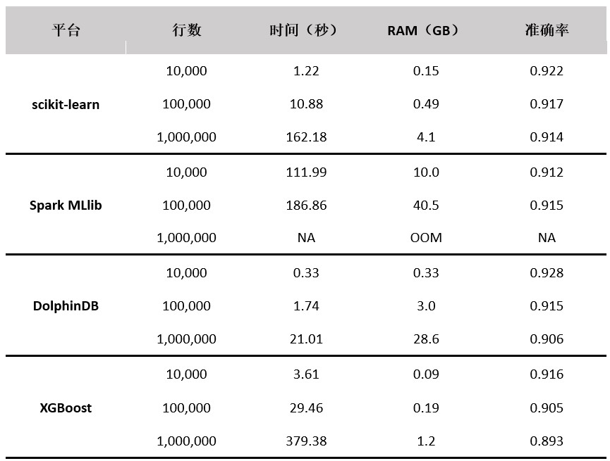
当树的数量为500,最大深度为10时,测试结果如下表所示:
当树的数量为500,最大深度为30时,测试结果如下表所示:
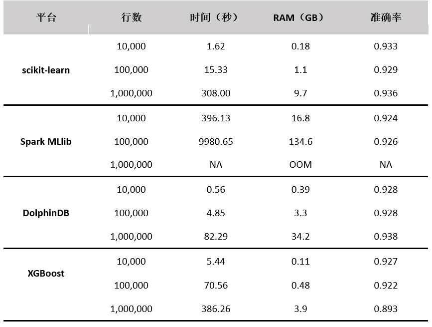
从准确率上看,Python scikit-learn、Spark MLlib和DolphinDB的准确率比较相近,略高于XGBoost的实现;从性能上看,从高到低依次为DolphinDB、Python scikit-learn、XGBoost、Spark MLlib。
在本次测试中,Python scikit-learn的实现使用了所有CPU核。
Spark MLlib的实现没有充分使用所有CPU核,内存占用最高,当数据量为10,000时,CPU峰值占用率约8%,当数据量为100,000时,CPU峰值占用率约为25%,当数据量为1,000,000时,它会因为内存不足而中断执行。
DolphinDB的实现使用了所有CPU核,并且它是所有实现中速度最快的,但内存占用是scikit-learn的2-7倍,是XGBoost的3-9倍。DolphinDB的随机森林算法实现提供了numJobs参数,可以通过调整该参数来降低并行度,从而减少内存占用。详情请参考DolphinDB用户手册。
XGBoost常用于boosted trees的训练,也能进行随机森林算法。它是算法迭代次数为1时的特例。XGBoost实际上在24线程左右时性能最高,其对CPU线程的利用率不如Python和DolphinDB,速度也不及两者。其优势在于内存占用最少。另外,XGBoost的具体实现也和其他平台的实现有所差异。例如,没有bootstrap这一过程,对数据使用无放回抽样而不是有放回抽样。这可以解释为何它的准确率略低于其它平台。
6.总结
Python scikit-learn的随机森林算法实现在性能、内存开销和准确率上的表现比较均衡,Spark MLlib的实现在性能和内存开销上的表现远远不如其他平台。DolphinDB的随机森林算法实现性能最优,并且DolphinDB的随机森林算法和数据库是无缝集成的,用户可以直接对数据库中的数据进行训练和预测,并且提供了numJobs参数,实现内存和速度之间的平衡。而XGBoost的随机森林只是迭代次数为1时的特例,具体实现和其他平台差异较大,最佳的应用场景为boosted tree。
附录
1.模拟生成数据的DolphinDB脚本
def genNormVec(cls, a, stdev, n) {\treturn norm(cls * a, stdev, n)}def genNormData(dataSize, colSize, clsNum, scale, stdev) {\tt = table(dataSize:0, `cls join (\u0026quot;col\u0026quot; + string(0..(colSize-1))), INT join take(DOUBLE,colSize))\tclassStat = groupby(count,1..dataSize, rand(clsNum, dataSize))\tfor(row in classStat){\t\tcls = row.groupingKey\t\tclassSize = row.count\t\tcols = [take(cls, classSize)]\t\tfor (i in 0:colSize)\t\t\tcols.append!(genNormVec(cls, scale, stdev, classSize))\t\ttmp = table(dataSize:0, `cls join (\u0026quot;col\u0026quot; + string(0..(colSize-1))), INT join take(DOUBLE,colSize))\t\tinsert into t values (cols)\t\tcols = NULL\t\ttmp = NULL\t}\treturn t}colSize = 50clsNum = 2t1m = genNormData(10000, colSize, clsNum, 2 / sqrt(20), 1.0)saveText(t1m, \u0026quot;t10k.csv\u0026quot;)t10m = genNormData(100000, colSize, clsNum, 2 / sqrt(20), 1.0)saveText(t10m, \u0026quot;t100k.csv\u0026quot;)t100m = genNormData(1000000, colSize, clsNum, 2 / sqrt(20), 1.0)saveText(t100m, \u0026quot;t1m.csv\u0026quot;)t1000 = genNormData(1000, colSize, clsNum, 2 / sqrt(20), 1.0)saveText(t1000, \u0026quot;t1000.csv\u0026quot;)2.Python scikit-learn的训练和预测脚本
import pandas as pdimport numpy as npfrom sklearn.ensemble import RandomForestClassifier, RandomForestRegressorfrom time import *test_df = pd.read_csv(\u0026quot;t1000.csv\u0026quot;)def evaluate(path, model_name, num_trees=500, depth=30, num_jobs=1): df = pd.read_csv(path) y = df.values[:,0] x = df.values[:,1:] test_y = test_df.values[:,0] test_x = test_df.values[:,1:] rf = RandomForestClassifier(n_estimators=num_trees, max_depth=depth, n_jobs=num_jobs) start = time() rf.fit(x, y) end = time() elapsed = end - start print(\u0026quot;Time to train model %s: %.9f seconds\u0026quot; % (model_name, elapsed)) acc = np.mean(test_y == rf.predict(test_x)) print(\u0026quot;Model %s accuracy: %.3f\u0026quot; % (model_name, acc))evaluate(\u0026quot;t10k.csv\u0026quot;, \u0026quot;10k\u0026quot;, 500, 10, 48) # choose your own parameter3.Spark MLlib的训练和预测代码
import org.apache.spark.mllib.tree.configuration.FeatureType.Continuousimport org.apache.spark.mllib.tree.model.{DecisionTreeModel, Node}object Rf { def main(args: Array[String]) = { evaluate(\u0026quot;/t100k.csv\u0026quot;, 500, 10) // choose your own parameter } def processCsv(row: Row) = { val label = row.getString(0).toDouble val featureArray = (for (i \u0026lt;- 1 to (row.size-1)) yield row.getString(i).toDouble).toArray val features = Vectors.dense(featureArray) LabeledPoint(label, features) } def evaluate(path: String, numTrees: Int, maxDepth: Int) = { val spark = SparkSession.builder.appName(\u0026quot;Rf\u0026quot;).getOrCreate() import spark.implicits._ val numClasses = 2 val categoricalFeaturesInfo = MapInt, Int val featureSubsetStrategy = \u0026quot;sqrt\u0026quot; val impurity = \u0026quot;gini\u0026quot;val maxBins = 32 val d_test = spark.read.format(\u0026quot;CSV\u0026quot;).option(\u0026quot;header\u0026quot;,\u0026quot;true\u0026quot;).load(\u0026quot;/t1000.csv\u0026quot;).map(processCsv).rdd d_test.cache() println(\u0026quot;Loading table (1M * 50)\u0026quot;) val d_train = spark.read.format(\u0026quot;CSV\u0026quot;).option(\u0026quot;header\u0026quot;,\u0026quot;true\u0026quot;).load(path).map(processCsv).rdd d_train.cache() println(\u0026quot;Training table (1M * 50)\u0026quot;) val now = System.nanoTime val model = RandomForest.trainClassifier(d_train, numClasses, categoricalFeaturesInfo, numTrees, featureSubsetStrategy, impurity, maxDepth, maxBins) println(( System.nanoTime - now )/1e9) val scoreAndLabels = d_test.map { point =\u0026gt; val score = model.trees.map(tree =\u0026gt; softPredict2(tree, point.features)).sum if (score * 2 \u0026gt; model.numTrees) (1.0, point.label) else (0.0, point.label) } val metrics = new MulticlassMetrics(scoreAndLabels) println(metrics.accuracy) } def softPredict(node: Node, features: Vector): Double = { if (node.isLeaf) { //if (node.predict.predict == 1.0) node.predict.prob else 1.0 - node.predict.prob node.predict.predict } else { if (node.split.get.featureType == Continuous) { if (features(node.split.get.feature) \u0026lt;= node.split.get.threshold) { softPredict(node.leftNode.get, features) } else { softPredict(node.rightNode.get, features) } } else { if (node.split.get.categories.contains(features(node.split.get.feature))) { softPredict(node.leftNode.get, features) } else { softPredict(node.rightNode.get, features) } } } } def softPredict2(dt: DecisionTreeModel, features: Vector): Double = { softPredict(dt.topNode, features) }}4.DolphinDB的训练和预测脚本
def createInMemorySEQTable(t, seqSize) {\tdb = database(\u0026quot;\u0026quot;, SEQ, seqSize)\tdataSize = t.size()\tts = ()\tfor (i in 0:seqSize) {\t\tts.append!(t[(i * (dataSize/seqSize)):((i+1)*(dataSize/seqSize))])\t}\treturn db.createPartitionedTable(ts, `tb)}def accuracy(v1, v2) {\treturn (v1 == v2).sum() \\ v2.size()}def evaluateUnparitioned(filePath, numTrees, maxDepth, numJobs) {\ttest = loadText(\u0026quot;t1000.csv\u0026quot;)\tt = loadText(filePath); clsNum = 2; colSize = 50\ttimer res = randomForestClassifier(sqlDS(\u0026lt;select * from t\u0026gt;), `cls, `col + string(0..(colSize-1)), clsNum, sqrt(colSize).int(), numTrees, 32, maxDepth, 0.0, numJobs)\tprint(\u0026quot;Unpartitioned table accuracy = \u0026quot; + accuracy(res.predict(test), test.cls).string())}evaluateUnpartitioned(\u0026quot;t10k.csv\u0026quot;, 500, 10, 48) // choose your own parameter5.XGBoost的训练和预测脚本
import pandas as pdimport numpy as npimport XGBoost as xgbfrom time import *def load_csv(path): df = pd.read_csv(path) target = df['cls'] df = df.drop(['cls'], axis=1) return xgb.DMatrix(df.values, label=target.values)dtest = load_csv('/hdd/hdd1/twonormData/t1000.csv')def evaluate(path, num_trees, max_depth, num_jobs): dtrain = load_csv(path) param = {'num_parallel_tree':num_trees, 'max_depth':max_depth, 'objective':'binary:logistic', 'nthread':num_jobs, 'colsample_bylevel':1/np.sqrt(50)} start = time() model = xgb.train(param, dtrain, 1) end = time() elapsed = end - start print(\u0026quot;Time to train model: %.9f seconds\u0026quot; % elapsed) prediction = model.predict(dtest) \u0026gt; 0.5 print(\u0026quot;Accuracy = %.3f\u0026quot; % np.mean(prediction == dtest.get_label()))evaluate('t10k.csv', 500, 10, 24) // choose your own parameter作者介绍
王一能,浙江智臾科技有限公司,重点关注大数据、时序数据库领域。
更多内容,请关注AI前线


 被折叠的 条评论
为什么被折叠?
被折叠的 条评论
为什么被折叠?
 到【灌水乐园】发言


