


 该博客文章介绍了如何使用Matlab解决叶片在0-1200秒内温度场随时间变化的瞬态传热问题。通过建立控制方程,设定边界条件,利用有限元方法进行网格划分和矩阵构建,最终得到温度变化的解。计算结果显示了全过程和1200s时的温度范围,并对比了稳态情况下的温度分布。
这一篇Blog是在A First course in FEM —— matlab代码实现求解传热问题(稳态) 基础上更进一步,求解瞬态传热问题。
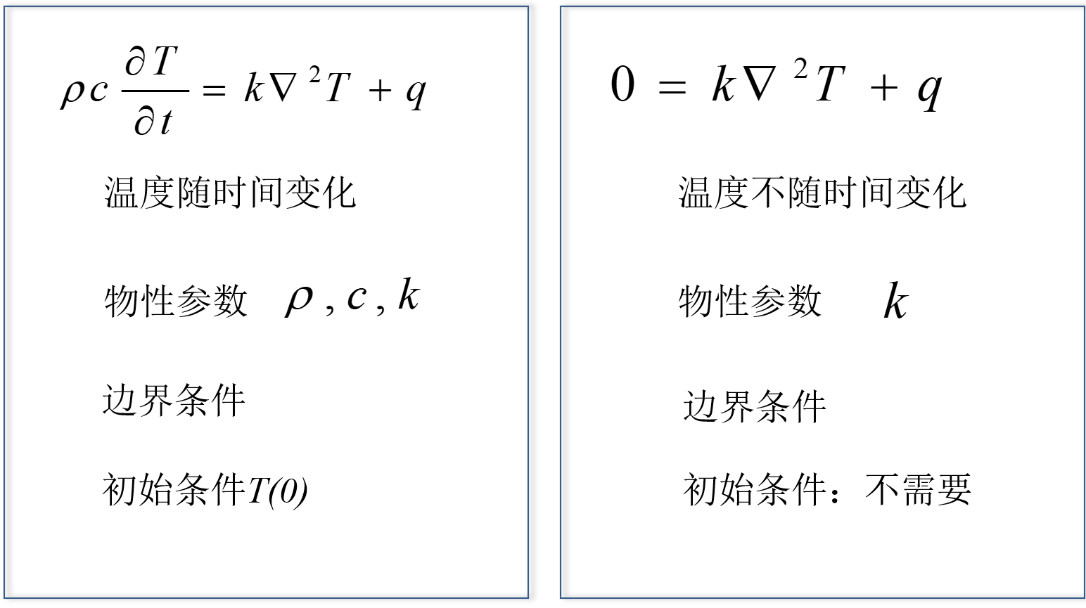
两者的区别如下图所示:
1. 问题描述
求解下图图所示叶片的温度场在[0-1200s]时间段内的变化,初始条件:T(0)=25℃。
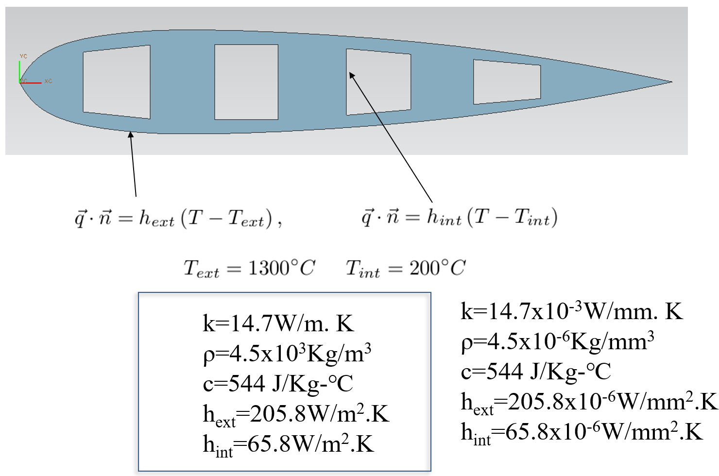
控制方程为:
2. 模型和网格
模型和网格设置详见A First course in FEM —— matlab代码实现求解传热问题(稳态)
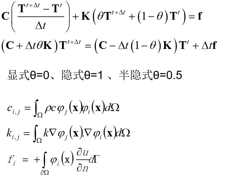
3. 系统矩阵
4. 代码实现
与稳态问题的代码框架一致。不同的代码如下:
bladeheat.m
% Clear variables

clear all;


% Set gas temperature and wall heat transfer coefficients at
% boundaries of the blade.  Note: Tcool(i) and hwall(i) are the
% values of Tcool and hwall for the ith boundary which are numbered
% as follows:
%
%   1 = external boundary (airfoil surface)
%   2 = 1st internal cooling passage (from leading edge)
%   3 = 2nd internal cooling passage (from leading edge)
%   3 = 3rd internal cooling passage (from leading edge)
%   3 = 4th internal cooling passage (from leading edge)


Tcool = [1573, 473, 473, 473, 473];
hwall = [205.8*10^-6, 65.8*10^-6, 65.8*10^-6, 65.8*10^-6, 65.8*10^-6];
k=14.7*10^-3;
ro= 4.5*10^-6;
c=544;

% Load in the grid file
% NOTE:  after loading a gridfile using the load(fname) command,
%        three important grid variables and data arrays exist.  These are:
%
% Nt: Number of triangles (i.e. elements) in mesh
%
% Nv: Number of nodes (i.e. vertices) in mesh
%
% Nbc: Number of edges which lie on a boundary of the computational
%      domain.
%
% tri2nod(3,Nt):  list of the 3 node numbers which form the current
%                 triangle.  Thus, tri2nod(1,i) is the 1st node of
%                 the i'th triangle, tri2nod(2,i) is the 2nd node
%                 of the i'th triangle, etc.
%
% xy(2,Nv): list of the x and y locations of each node.  Thus,
%           xy(1,i) is the x-location of the i'th node, xy(2,i)
%           is the y-location of the i'th node, etc.
%
% bedge(3,Nbc): For each boundary edge, bedge(1,i) and bedge(2,i)
%               are the node numbers for the nodes at the end
%               points of the i'th boundary edge.  bedge(3,i) is an
%               integer which identifies which boundary the edge is
%               on. In this solver, the third value has the
%               following meaning:
%
%               bedge(3,i) = 0: edge is on the airfoil
%               bedge(3,i) = 1: edge is on the first cooling passage
%               bedge(3,i) = 2: edge is on the second cooling passage
%               bedge(3,i) = 3: edge is on the third cooling passage
%               bedge(3,i) = 4: edge is on the fourth cooling passage
%
bladeread;


% Start timer
Time0 = cputime;

% Zero stiffness matrix

K = zeros(Nv, Nv);
b = zeros(Nv, 1);
C= zeros(Nv, Nv);
% Zero maximum element size
hmax = 0;


% Loop over elements and calculate residual and stiffness matrix

for ii = 1:Nt,

  kn(1) = tri2nod(1,ii);
  kn(2) = tri2nod(2,ii);
  kn(3) = tri2nod(3,ii);

  xe(1) = xy(1,kn(1));
  xe(2) = xy(1,kn(2));
  xe(3) = xy(1,kn(3));

  ye(1) = xy(2,kn(1));
  ye(2) = xy(2,kn(2));
  ye(3) = xy(2,kn(3));

  % Calculate circumcircle radius for the element
  % First, find the center of the circle by intersecting the median
  % segments from two of the triangle edges.

  dx21 = xe(2) - xe(1);
  dy21 = ye(2) - ye(1);

  dx31 = xe(3) - xe(1);
  dy31 = ye(3) - ye(1);

  x21  = 0.5*(xe(2) + xe(1));
  y21  = 0.5*(ye(2) + ye(1));

  x31  = 0.5*(xe(3) + xe(1));
  y31  = 0.5*(ye(3) + ye(1));

  b21 = x21*dx21 + y21*dy21;
  b31 = x31*dx31 + y31*dy31;

  xydet = dx21*dy31 - dy21*dx31;

  x0 = (dy31*b21 - dy21*b31)/xydet;
  y0 = (dx21*b31 - dx31*b21)/xydet;

  Rlocal = sqrt((xe(1)-x0)^2 + (ye(1)-y0)^2);

  if (hmax < Rlocal),
    hmax = Rlocal;
  end

  % Calculate all of the necessary shape function derivatives, the
  % Jacobian of the element, etc.

  % Derivatives of node 1's interpolant
  dNdxi(1,1) = -1.0; % with respect to xi1
  dNdxi(1,2) = -1.0; % with respect to xi2

  % Derivatives of node 2's interpolant
  dNdxi(2,1) =  1.0; % with respect to xi1
  dNdxi(2,2) =  0.0; % with respect to xi2

  % Derivatives of node 3's interpolant
  dNdxi(3,1) =  0.0; % with respect to xi1
  dNdxi(3,2) =  1.0; % with respect to xi2

  % Sum these to find dxdxi (note: these are constant within an element)
  dxdxi = zeros(2,2);
  for nn = 1:3
    dxdxi(1,:) = dxdxi(1,:) + xe(nn)*dNdxi(nn,:);
    dxdxi(2,:) = dxdxi(2,:) + ye(nn)*dNdxi(nn,:);
  end

  % Calculate determinant for area weighting
  J = dxdxi(1,1)*dxdxi(2,2) - dxdxi(1,2)*dxdxi(2,1);
  A = 0.5*abs(J); % Area is half of the Jacobian

  % Invert dxdxi to find dxidx using inversion rule for a 2x2 matrix
  dxidx = [ dxdxi(2,2)/J, -dxdxi(1,2)/J; ...
	   -dxdxi(2,1)/J,  dxdxi(1,1)/J];

  % Calculate dNdx
  dNdx = dNdxi*dxidx;    %lian shi fa ze

  % Add contributions to stiffness matrix for node 1 weighted residual
  K(kn(1), kn(1)) = K(kn(1), kn(1)) + k*(dNdx(1,1)*dNdx(1,1) + dNdx(1,2)*dNdx(1,2))*A;  %2*1/2A
  K(kn(1), kn(2)) = K(kn(1), kn(2)) + k*(dNdx(1,1)*dNdx(2,1) + dNdx(1,2)*dNdx(2,2))*A;
  K(kn(1), kn(3)) = K(kn(1), kn(3)) + k*(dNdx(1,1)*dNdx(3,1) + dNdx(1,2)*dNdx(3,2))*A;

  % Add contributions to stiffness matrix for node 2 weighted residual
  K(kn(2), kn(1)) = K(kn(2), kn(1)) + k*(dNdx(2,1)*dNdx(1,1) + dNdx(2,2)*dNdx(1,2))*A;
  K(kn(2), kn(2)) = K(kn(2), kn(2)) + k*(dNdx(2,1)*dNdx(2,1) + dNdx(2,2)*dNdx(2,2))*A;
  K(kn(2), kn(3)) = K(kn(2), kn(3)) + k*(dNdx(2,1)*dNdx(3,1) + dNdx(2,2)*dNdx(3,2))*A;

  % Add contributions to stiffness matrix for node 3 weighted residual
  K(kn(3), kn(1)) = K(kn(3), kn(1)) + k*(dNdx(3,1)*dNdx(1,1) + dNdx(3,2)*dNdx(1,2))*A;
  K(kn(3), kn(2)) = K(kn(3), kn(2)) + k*(dNdx(3,1)*dNdx(2,1) + dNdx(3,2)*dNdx(2,2))*A;
  K(kn(3), kn(3)) = K(kn(3), kn(3)) + k*(dNdx(3,1)*dNdx(3,1) + dNdx(3,2)*dNdx(3,2))*A;

  %C矩阵
  C(kn(1), kn(1)) = C(kn(1), kn(1)) + ro*c*A/6;
  C(kn(1), kn(2)) = C(kn(1), kn(2)) + ro*c*A/12;
  C(kn(1), kn(3)) = C(kn(1), kn(3)) + ro*c*A/12;

  C(kn(2), kn(1)) = C(kn(2), kn(1)) + ro*c*A/12;
  C(kn(2), kn(2)) = C(kn(2), kn(2)) + ro*c*A/6;
  C(kn(2), kn(3)) = C(kn(2), kn(3)) + ro*c*A/12;

  C(kn(3), kn(1)) = C(kn(3), kn(1)) + ro*c*A/12;
  C(kn(3), kn(2)) = C(kn(3), kn(2)) + ro*c*A/12;
  C(kn(3), kn(3)) = C(kn(3), kn(3)) + ro*c*A/6;

end


% Loop over boundary edges and account for bc's
% Note: the bc's are all convective heat transfer coefficient bc's
% so the are of 'Robin' form.  This requires modification of the
% stiffness matrix as well as impacting the right-hand side, b.
%

for ii = 1:Nbc,

  % Get node numbers on edge
  kn(1) = bedge(1,ii);
  kn(2) = bedge(2,ii);

  % Get node coordinates
  xe(1) = xy(1,kn(1));
  xe(2) = xy(1,kn(2));

  ye(1) = xy(2,kn(1));
  ye(2) = xy(2,kn(2));

  % Calculate edge length
  ds = sqrt((xe(1)-xe(2))^2 + (ye(1)-ye(2))^2);

  % Determine the boundary number
  bnum = bedge(3,ii) + 1;

  % Based on boundary number, set heat transfer bc
  K(kn(1), kn(1)) = K(kn(1), kn(1)) + hwall(bnum)*ds*(1/3);
  K(kn(1), kn(2)) = K(kn(1), kn(2)) + hwall(bnum)*ds*(1/6);
  b(kn(1))        = b(kn(1))        + hwall(bnum)*ds*0.5*Tcool(bnum);

  K(kn(2), kn(1)) = K(kn(2), kn(1)) + hwall(bnum)*ds*(1/6);
  K(kn(2), kn(2)) = K(kn(2), kn(2)) + hwall(bnum)*ds*(1/3);
  b(kn(2))        = b(kn(2))        + hwall(bnum)*ds*0.5*Tcool(bnum);

end

%确定Tsol维度
timetot=1200;
dt=10;
n=fix(timetot/dt);
Tsol=298*ones(Nv,n+1);

%methode to run
theta=0.5;

% Solve for temperature
for i=1:n
    Tsol(:,i+1)=inv(C+dt.*theta.*K)*((C-dt.*(1-theta).*K)*Tsol(:,i)+dt.*b);
end
Tmax = max(max(Tsol));
Tmin = min(min(Tsol));
Tmaxx = max(max(Tsol(:,n+1)));
Tminn = min(min(Tsol(:,n+1)));
% Finish timer
Time1 = cputime;

% Plot solution
bladeplot;

% Report outputs


fprintf('Number of nodes      = %i\n',Nv);
fprintf('Number of elements   = %i\n',Nt);
fprintf('Maximum element size = %5.3f\n',hmax);
fprintf('Minimum temperature  = %6.1f\n',Tmin);
fprintf('Maximum temperature  = %6.1f\n',Tmax);
fprintf('Minimum temperature at last  = %6.1f\n',Tminn);
fprintf('Maximum temperature at last = %6.1f\n',Tmaxx);
fprintf('CPU Time (secs)      = %f\n',Time1 - Time0);
bladeplot.m
% Plot T in triangles
v=VideoWriter('transientblade.avi');
open(v);
f=10;num=fix(n/f);
for i=0:num-1
for ii = 1:Nt
  for nn = 1:3
    xtri(nn,ii) = xy(1,tri2nod(nn,ii));
    ytri(nn,ii) = xy(2,tri2nod(nn,ii));
    Ttri(nn,ii) = Tsol(tri2nod(nn,ii),1+f*i);
  end
end
figure;
HT = patch(xtri,ytri,Ttri);
axis('equal');
set(HT,'LineStyle','none');
title('Temperature(K)');
caxis([298,1573]);
HC = colorbar;
colormap(jet);
hold on; bladeplotgrid; hold off;
frame(i+1)=getframe;
end
writeVideo(v,frame);
close(v);
5. 计算结果
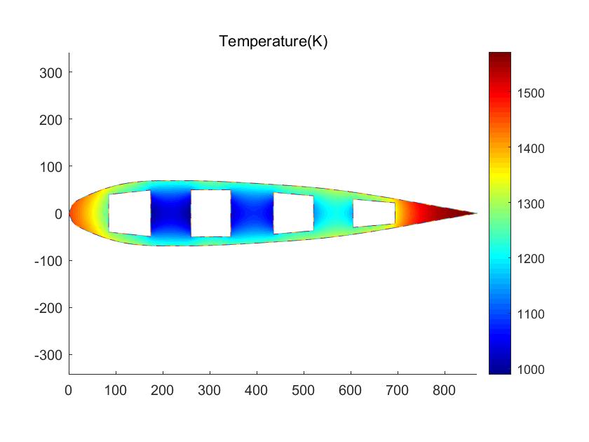
全过程最低温度= 282.1 K
全过程最高温度 = 1572.1 K
1200s时最低温度 = 1013.0 K
1200s时最高温度 = 1572.1 K
1200S时温度分布如下图,与稳态时的温度分布相近。


 607
607

 被折叠的 条评论
为什么被折叠?
被折叠的 条评论
为什么被折叠?
 到【灌水乐园】发言


