


图数据库 graph
Earlier this year, I published several articles on SQLShack with an aim of demonstrating tools available for visualising SQL Server 2017 graph databases. I was so caught up in the excitement of having SQL Server finally support graph databases that I forgot that some people still do not have a good grasp of how graph databases work let alone consider replacing their relational databases models in favour of graph. Although there are several ways that one can go about explaining the usefulness of graph databases over its relational counterpart, I have opted to focus on the benefits and strengths of graph databases by demonstrating the differences in which graph and relational databases deal with hierarchical datasets.
今年早些时候,我在SQLShack上发表了几篇文章,目的是演示可用于可视化SQL Server 2017图形数据库的工具。 令SQL Server最终支持图数据库的激动使我非常着迷,以至于我忘记了有些人仍然对图数据库的工作原理不甚了解,更不用说考虑用关系图代替关系数据库模型了。 尽管可以通过多种方法来解释图数据库相对于关系数据库的有用性,但我还是通过展示图和关系数据库处理分层数据集的差异来重点关注图数据库的优点和优势。
分层数据集的案例: 足球运动员与经理的关系 (The Case for Hierarchical Datasets: Footballer-Manager Relationship)
Hierarchical datasets are often synonymous with tree-like data structures and at one point or another, we’ve all been part of hierarchical data structures; be at places of work through employee-manager relationships, in our homes via child-parent relationships or through our levels of friendships on online social media platforms. The hierarchical relationship that I want to look at in this article is the Footballer-Manager relationship and how such a relationship can be represented in both graph and relational databases.
分层数据集通常是树状数据结构的同义词,在某一点或另一点,我们都属于分层数据结构的一部分。 通过员工与经理的关系,通过子女与父母的关系在家中或通过在线社交媒体平台上的友谊水平来工作。 我想在本文中探讨的层次关系是Footballer-Manager关系,以及如何在图形数据库和关系数据库中表示这种关系。
Figure 1 depicts a Footballer-Manager hierarchical relationship between players that – at some point – were part of the Spanish La Liga club, Atlético Madrid. As it can be seen in Figure 1, the majority of Footballer-Manager relationships are between manager Gregorio Manzano and players Gabi, Rubén Olivera, and Kiki Musampa. Whilst Diego Simeone was at some point managed by Gregorio Manzano, he has gone on to manage players of his own including the likes of Diego Costa, Gabi and Juanfran.
图1描绘了球员之间足球运动员-经理之间的等级关系,在某种程度上,他们是西班牙西甲俱乐部马德里竞技的一部分。 由于它可以在图1中可以看出,大多数足球-经理关系是经理格雷戈里奥·曼萨诺和球员加比 , 奥利维拉和基基·马桑帕之间。 尽管迭戈·西蒙内在某个时候由格雷戈里奥·曼萨诺 ( Gregorio Manzano)管理,但他继续管理自己的球员,包括像迭戈·科斯塔 ( Diego Costa),加比(Gabi)和胡安弗兰(Juanfran)这样的球员。
The information represented in Figure 1 can be modelled for both relational and graph databases. Consequently, I’ve gone ahead and produced such models as shown in Figure 2 wherein the left-hand side of the black vertical bar represents the relational database model whilst the other side represents the graph. Noticeably in both models is the fact that the FootballerManager entity has a relationship with itself – what is often called a self-join.
图1中表示的信息可以为关系数据库和图形数据库建模。 因此,我继续制作了如图2所示的模型,其中黑色竖条的左侧代表关系数据库模型,而另一侧则代表图形。 值得注意的是,在这两个模型中, FootballerManager实体与自身都有关系-通常称为自联接。
One significant difference in Figure 2 is the way self-joined relationships are indicated. For instance, keys are used in the relational model to denote relationships such that the foreign key links back to its primary key. Graph databases, on the other hand, take an entirely different approach to representing relationships. This is because, in graph databases, relationships are stored as standalone tables and thus the managedBY relationship is a standalone table separate to the FootballerManager entity. In other words, for every entity-relationship that you define in a graph database, a separate standalone table is created to store such a relationship. To demonstrate this argument, we’ve used information from Figure 2 to create a logical entity-relationship-diagram (ERD), shown in Figure 3. Again, the left-hand side of the black vertical bar in Figure 3 represents logical ERD for the relational database whilst the right-hand side signifies graph.
图2中的一个重要区别是表示自联接关系的方式。 例如,键在关系模型中用于表示关系,以使外键链接回其主键。 另一方面,图形数据库采用完全不同的方法来表示关系。 这是因为在图形数据库中,关系存储为独立表,因此managedBY关系是独立于FootballerManager实体的独立表。 换句话说,对于在图形数据库中定义的每个实体关系,都会创建一个单独的独立表来存储这种关系。 为了证明这一观点,我们使用了图2中的信息来创建逻辑实体-关系图(ERD),如图3所示。 同样, 图3中黑色竖线的左侧代表关系数据库的逻辑ERD,而右侧则代表图形。
As per the total number of objects in Figure 3, graph database creates more physical objects than its relational counterpart. This means that we should expect the exercise of creating and populating objects in a graph database to be quite lengthier than a relational database. However – as it will be demonstrated later – all of your object-creation and populating efforts get rewarded later-on during data retrieval exercise as it is generally faster to retrieve hierarchical data out of graph compared to relational databases.
根据图3中的对象总数,图数据库创建的物理对象比其关系对应的对象更多。 这意味着我们应该期望在图形数据库中创建和填充对象的工作比关系数据库要长得多。 但是,正如稍后将要演示的那样,在数据检索过程中,您的所有对象创建和填充工作都会在以后获得回报,因为与关系数据库相比,从图形中检索层次结构数据通常更快。
衡量查询性能:关系数据库与图形数据库 (Measuring Query Performance: Relational Databases vs. Graph Databases)
In this section, we compare query performances for both relational and graph databases by creating physical tables based on logical ERD design shown in Figure 3.
在本节中,我们通过基于图3所示的逻辑ERD设计创建物理表,比较关系数据库和图形数据库的查询性能。
Measuring Relational Database Query Performance
衡量关系数据库查询性能
According to our ERD diagram for the relational database, we need to create only a single table – FootballerManager. I have gone ahead and created and populated such a table as shown in Figure 4 – (A database backup containing all tables used in this demo is available under the Downloads section at the bottom of this article).
根据关系数据库的ERD图,我们只需要创建一个表– FootballerManager 。 我已经继续创建并填充了这样一个表, 如图4所示-(包含此演示中使用的所有表的数据库备份位于本文底部的“ 下载”部分下)。
Figure 4
图4Having created and populated our table, we next move on to querying the table using Script 1.
创建并填充了表格后,接下来我们继续使用脚本1查询表格。
SELECT e.[Name] AS 'Manager',
       m.[Name] AS 'Player'
FROM [dbo].[FootballerManager] e,
     [dbo].[FootballerManager] m
WHERE e.[PlayerID] = m.[ManagedByID]
      AND e.[Name] = 'Diego Simeone';
The results of Script 1 execution are shown in Figure 5 – which basically returns a list of all players managed by Diego Simeone.
脚本1执行的结果如图5所示-基本上返回了Diego Simeone管理的所有玩家的列表。
Figure 5
图5Furthermore, using ApexSQL Plan I’ve gone ahead and generated an execution plan for Script 1. Notice in the generated execution plan in Figure 6 that the majority of Script 1 execution was spent performing hash match joins.
此外,使用ApexSQL Plan 我已经为脚本1生成了执行计划。 请注意,在图6所生成的执行计划中, 脚本1的大部分执行都花费在执行哈希匹配联接上。
Figure 6 图6 Hash match joins often indicate TempDB activity and as indicated in the query’s IO statistics shown in Figure 7, the SQL Server optimizer made use of Workfile and Worktable temporary objects to identify correct combinations that will satisfy query conditions stipulated in Script 1.
哈希联接比赛往往表明tempdb活动,并如在图7所示的查询的IO统计表明,SQL Server优化利用工作文件和工作台临时对象,以确定正确的组合,将满足查询条件的脚本1规定。
Figure 7 图7 Measuring Graph Database Query Performance
测量图数据库查询性能
Script 2 is graph database query version of Script 1.
脚本2是脚本1的图形数据库查询版本。
SELECT person1.name AS 'Manager',
       person2.name AS 'Player'
FROM Footballer person1,
     Footballer person2,
     managedby
WHERE MATCH(person1-(managedby)->person2)
      AND person1.name = 'Diego Simeone';
Script 2 剧本2 The execution of Script 2 returns an output similar to what is shown in Figure 5 but as expected this version of the query in a graph database uses an entirely different execution plan to that of a relational database query.
脚本2的执行返回的输出类似于图5中所示的输出,但是正如预期的那样,图形数据库中的该版本的查询使用与关系数据库查询完全不同的执行计划。
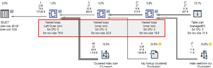
Figure 8 图8 Figure 8 shows execution plan of Script 2. The execution plan indicates that the graph database query relied on nested loop joins instead of hash match joins used in the relational database version of the query. Nested loops basically identify matches by taking each record from the outer input and applying it against the inner input. In this case, our managedBY relationship table is the outer input being applied against the Footballer table. The predicate “Diego Simeone” reduces the size of our outer input from 27 to 3 – as 3 is the total number of records (relationships) linked to Diego Simeone. Now when we go looking for the names of the players linked to Diego Simeone, we only scan the Footballer table against 3 relationships instead of 27. So, the formula for our nested loop becomes 3*22 (number of possible player names) instead of 27 * 22.
图8显示了脚本2的执行计划。 执行计划表明,图数据库查询依赖于嵌套循环联接,而不是查询的关系数据库版本中使用的哈希匹配联接。 嵌套循环基本上通过从外部输入中获取每个记录并将其应用于内部输入来标识匹配项。 在这种情况下,我们的managedBY关系表是对Footballer表应用的外部输入。 谓词“ Diego Simeone ”将外部输入的大小从27减少到3 –因为3是与Diego Simeone相关的记录(关系)的总数。 现在,当我们查找链接到Diego Simeone的球员的姓名时,我们仅针对3个关系而不是27个关系来扫描Footballer表。因此,嵌套循环的公式变为3 * 22(可能的球员姓名数),而不是27 * 22。
摘要 (Summary)
Hierarchical datasets easily highlight the modelling and query execution differences in both relational and graph databases. However, this is by no means an indication that you should start throwing away the one database system over the other. Graph databases are more efficient when data relationships are at the core of your requirement. Below is a list of some key differences between Relational and Graph databases. We conclude this article by summarising some of the key differences between relational databases and graph databases.
层次数据集可以轻松突出关系数据库和图形数据库中的建模和查询执行差异。 但是,这绝不表示您应该开始抛弃一个数据库系统而取代另一个数据库系统。 当数据关系是您的核心要求时,图形数据库将更加高效。 下面列出了关系数据库和图数据库之间的一些关键区别。 我们通过总结关系数据库和图形数据库之间的一些关键区别来结束本文。
| Relational Database | Graph Database |
| Entity Relationships exist as keys within dataset | Entity Relationships are represented as tables |
| Increase in size of dataset reduces query performance | Increase in connections/relationships degrades query performance |
| Harder to introduce new relationships/keys as it requires altering definition of underlying table | Easy to add new relationships |
| 关系型数据库 | 图数据库 |
| 实体关系作为数据集中的键存在 | 实体关系表示为表格 |
| 数据集大小的增加会降低查询性能 | 连接/关系的增加会降低查询性能 |
| 难以引入新的关系/键,因为它需要更改基础表的定义 | 轻松添加新关系 |
资料下载 (Downloads)
参考资料 (References)
- Graph processing with SQL Server and Azure SQL Database 使用SQL Server和Azure SQL数据库进行图形处理
- Hash Match – SQL Server Graphical Execution Plan 哈希匹配– SQL Server图形执行计划
- Hierarchical database model 分层数据库模型
图数据库 graph


 546
546

 被折叠的 条评论
为什么被折叠?
被折叠的 条评论
为什么被折叠?
 到【灌水乐园】发言


