


In this post we continue looking at the Cardinality Estimator (CE). The article explores some join estimation algorithms in the details, however this is not a comprehensive join estimation analysis, the goal of this article is to give a reader a flavor of join estimation in SQL Server.
在本文中,我们继续研究基数估计器(CE)。 本文详细探讨了一些联接估计算法,但这并不是一个全面的联接估计分析,本文的目的是使读者了解SQL Server中的联接估计。
The complexity of the CE process is that it should predict the result without any execution (at least in the current versions), in other words it should somehow model the real execution and based on that modeling get the number of rows. Depending on the chosen model the predicted result may be closer to the real one or not. One model may give very good results in one type of situations, but will fail in the other, the second one may fail the first set and succeed in the second one. That is why SQL server uses different approaches when estimating different types of operations with different properties. Joins are no exception to this.
CE流程的复杂性在于它应该预测结果而不执行任何操作(至少在当前版本中是如此),换句话说,它应该以某种方式对实际执行进行建模,并基于该建模获得行数。 根据所选模型,预测结果可能会更接近真实结果。 一个模型在一种情况下可能会给出很好的结果,但在另一种情况下会失败,第二种模型可能会在第一种情况下失败并在第二种情况下成功。 这就是为什么SQL Server在估计具有不同属性的不同类型的操作时使用不同的方法的原因。 联接也不例外。
演示 (The Demos)
If you wish to follow this post executing scripts or test it yourself, below is the description of what we are using here. We use DB AdventureworksDW2016CTP3 and we use COMPATIBILITY_LEVEL setting to test SQL Server 2014 behavior (CE 120) and SQL Server 2016 behavior (CE 130).
如果您希望按照此后执行脚本或自己进行测试,则以下是我们在此处使用的描述。 我们使用DB AdventureworksDW2016CTP3,并使用COMPATIBILITY_LEVEL设置来测试SQL Server 2014行为(CE 120)和SQL Server 2016行为(CE 130)。
For the demonstration purposes, we use two not officially documented, but well documented over the internet, trace flags (TFs):
出于演示目的,我们使用两个未正式记录但在互联网上有据可查的跟踪标记(TF):
- 3604 – Directs SQL Server output to console (Message window in SQL Server Management Studio (SSMS)) 3604 –将SQL Server输出定向到控制台(SQL Server Management Studio(SSMS)中的“消息”窗口)
- 2363 – Starting from SQL Server 2014 outputs information about the estimation process 2363 –从SQL Server 2014开始,输出有关估计过程的信息
We are talking about estimations and we don’t actually need to execute the query, so don’t press “Execute” in SSMS otherwise a server will cache the query plan and we don’t need this. To compile a query and not to cache it, just press “Display Estimated Execution Plan” icon or press CTRL + L in SSMS.
我们正在谈论估计,实际上我们不需要执行查询,因此不要在SSMS中按“执行”,否则服务器将缓存查询计划,因此我们不需要这样做。 要编译查询而不缓存查询,只需按“显示估计的执行计划”图标或在SSMS中按CTRL +L。
Finally, we will switch to the AdventureworksDW2016CTP3 DB and clear server cache, I assume all the code below is located on the test server only.
最后,我们将切换到AdventureworksDW2016CTP3 DB并清除服务器缓存,假设下面的所有代码仅位于测试服务器上 。
use AdventureworksDW2016CTP3;
dbcc freeproccache;
go
SQL Server中的联接估计策略 (Join Estimation Strategies in SQL Server)
During databases evolution (about half a century now) there were a lot of approaches how to estimate a JOIN, described in numerous research papers. Each DB vendor makes its own twists and improvements to classical algorithms or develops its own. In case of SQL Server these algorithms are proprietary and not public, so we can’t know all the details, however general things are documented. With that knowledge, and some patience, we can figure out some interesting things about the join estimation process.
在数据库发展过程中(大约半个世纪了),许多研究论文都介绍了许多估算JOIN的方法。 每个数据库供应商都会对经典算法做出自己的曲折和改进,或者自己开发。 对于SQL Server,这些算法是专有的而不是公开的,因此我们无法了解所有详细信息,但已记录了一般性内容。 有了这些知识和一些耐心,我们可以找出有关联接估计过程的一些有趣的事情。
If you recall my blog post about CE 2014 you may remember that the estimation process in the new framework is done with the help of such things as calculators – algorithms encapsulated into the classes and methods, the particular one is chosen for the estimation depending on the situation.
如果您还记得我关于CE 2014的博客文章 ,您可能还记得新框架中的估算过程是借助计算器(封装在类和方法中的算法)的帮助下完成的,因此,根据具体情况选择特定的估算方法。情况。
In this post we will look at two different join estimation strategies:
在本文中,我们将研究两种不同的联接估计策略:
- Histogram Join 直方图连接
- Simple Join 简单加入
直方图连接 (Histogram Join)
Let’s switch to CE 120 (SQL Server 2014) using a compatibility level and consider the following query.
让我们使用兼容级别切换到CE 120(SQL Server 2014),并考虑以下查询。
Execute:
执行:
alter database [AdventureworksDW2016CTP3] set compatibility_level = 120;
Display Estimated Execution Plan:
显示估算的执行计划:
select
	*
from
	dbo.FactInternetSales fis
	join dbo.DimDate dc on fis.ShipDateKey = dc.DateKey
option(querytraceon 3604, querytraceon 2363);
SQL Server uses this calculator in many other cases, and this output is not very informative in the meaning of how the JOIN is estimated. In fact, SQL Server has at least two options:
SQL Server在许多其他情况下都使用此计算器,并且此输出在如何估计JOIN的意义上不是很有帮助。 实际上,SQL Server至少有两个选择:
- Coarse Histogram Estimation 粗直方图估计
- Step-by-step Histogram Estimation 逐步直方图估计
The first one is used in the new CE in SQL Server 2014 and 2016 by default. The second one is used by the earlier CE mechanism.
默认情况下,第一个用于SQL Server 2014和2016中的新CE。 第二种由早期的CE机制使用。
Step-by-step Histogram Estimation in the earlier versions used histogram alignment with step linear interpolation. The description of the general algorithm is beyond the scope of this article, however, if you are interested, I’ll refer you to the Nicolas’s Bruno (Software Developer, Microsoft) work “Statistics on Query Expressions in Relational Database Management Systems” COLUMBIA UNIVERSITY, 2003. And to give you the flavor of what’s going on, I’ll post an image from this work here:
早期版本中的逐步直方图估计使用直方图对齐和逐步线性插值。 通用算法的描述不在本文讨论范围之内,但是,如果您有兴趣,我将带您参考Nicolas的Bruno( Microsoft软件开发人员 )的工作“关系数据库管理系统中查询表达式的统计信息”哥伦比亚大学,2003年。为了让您了解正在发生的事情,我将在此处发布此工作的图像:
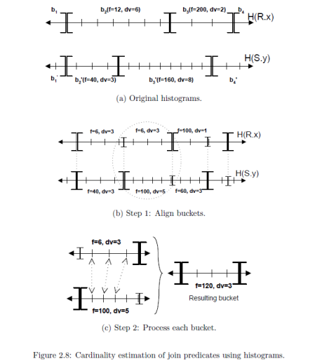
This is a general algorithm that gives an idea about how it works. As I have already mentioned, real algorithms are proprietary and not publicly available.
这是一种通用算法,可提供有关其工作原理的想法。 正如我已经提到的,真实算法是专有的,并且不公开可用。
Coarse Histogram Estimation is a new algorithm and less documented, even in terms of general concepts. It is known that instead of aligning histograms step by step, it aligns them with only minimum and maximum histogram boundaries. This method potentially introduces less CE mistakes (not always however, because we remember that this is just a model). Now we will observe how it looks like inside SQL Server, for that purpose, we need to attach WinDbg with public symbols for SQL Server 2016 RTM.
粗直方图估计是一种新算法,即使在一般概念方面,其文献资料也很少。 众所周知,与其一步一步地对齐直方图,不如将其与最小和最大直方图边界对齐。 这种方法可能会引入较少的CE错误(但是并非总是如此,因为我们记住这只是一个模型)。 现在,我们将观察它在SQL Server内部的外观,为此,我们需要为WinDbg附加SQL Server 2016 RTM的公共符号。
Coarse alignment is the default algorithm under compatibility level higher than 110, and what we see in WinDbg in SQL Server 2016 is:
粗调是兼容性级别高于110时的默认算法,我们在SQL Server 2016的WinDbg中看到的是:
The breakpoint on the method CHistogramWalker_Coarse::ExtractStepStats is reached twice while optimizing the query above, because we have two histograms that are used for a join estimation and each of them are aligned in the coarse manner described above.
在优化上面的查询时,方法CHistogramWalker_Coarse :: ExtractStepStats的断点达到了两次,因为我们有两个直方图用于连接估计,并且每个直方图都以上述粗略方式对齐。
To take a step further, I also put a break point on the method CHistogramWalker_Coarse::FAdvance, which is also invoked twice, but before the ExtractStepStats, doing some preparation work. I stepped through it and examined some processor registers.
为了更进一步,我还在方法CHistogramWalker_Coarse :: FAdvance上设置了一个断点,该方法也被调用了两次,但在ExtractStepStats之前进行了一些准备工作。 我逐步浏览了一下并检查了一些处理器寄存器。

ASM command MOVSD moves the value 401412c160000000 from memory to the register xmm5 for some further manipulations. If you are wondering what is so special about this value, you may use hex to double calculator to convert this to double (I’m using this one):
ASM命令MOVSD将值401412c160000000从内存移动到寄存器xmm5,以进行进一步的操作。 如果您想知道此值有什么特别之处,可以使用十六进制double计算器将其转换为double(我正在使用此值 ):
Now let’s ask DBCC STATISTICS for the histogram statistics for the table’s FactInternetSales join column, in my case this statistic is named _WA_Sys_00000004_276EDEB3.
现在,让我们向DBCC STATISTICS查询表的FactInternetSales连接列的直方图统计信息,在我的情况下,此统计信息名为_WA_Sys_00000004_276EDEB3。
dbcc show_statistics(FactInternetSales, _WA_Sys_00000004_276EDEB3) with histogram;
The result is:
结果是:
Look at the very first histogram row of the column that contains rows equal to the histogram upper boundary. This is the exact rounded value that was loaded by the method CHistogramWalker_Coarse::FAdvance before step estimation. If you spend more time in WInDbg you may figure out what exactly values are loaded then and what happens to them, but that is not the subject of this article and in my opinion is not so important. More important is the knowledge that there is a new default join histogram estimation algorithm that uses the minimum and maximum boundaries and it really works in this fashion.
查看列的第一个直方图行,其中包含等于直方图上限的行。 这是在步估计之前由方法CHistogramWalker_Coarse :: FAdvance加载的精确舍入值。 如果您花更多时间在WInDbg上,则可能会弄清楚到底是加载了什么值以及它们发生了什么,但这不是本文的主题,我认为并不是那么重要。 更重要的是,要知道存在一种新的默认联接直方图估计算法,该算法使用最小和最大边界,并且确实可以这种方式工作。
Finally, let’s enable an actual execution plan to see the difference between actual rows and estimated rows, and run the query under different compatibility levels.
最后,让我们启用一个实际的执行计划,以查看实际行与估计行之间的差异,并在不同的兼容性级别下运行查询。
alter database [AdventureworksDW2016CTP3] set compatibility_level = 110;
go
select
	*
from
	dbo.FactInternetSales fis
	join dbo.DimDate dc on fis.ShipDateKey = dc.DateKey;
go
alter database [AdventureworksDW2016CTP3] set compatibility_level = 120;
go
select
	*
from
	dbo.FactInternetSales fis
	join dbo.DimDate dc on fis.ShipDateKey = dc.DateKey;
go
alter database [AdventureworksDW2016CTP3] set compatibility_level = 130;
go
select
	*
from
	dbo.FactInternetSales fis
	join dbo.DimDate dc on fis.ShipDateKey = dc.DateKey;
go
The results are:
结果是:
As we can see both CE 120 (SQL Server 2014) and CE 130 (SQL Server 2016) use Coarse Alignment and it is an absolute winner in this round. The old CE underestimates about 30% of the rows.
正如我们所看到的,CE 120(SQL Server 2014)和CE 130(SQL Server 2016)都使用粗调,它是本轮的绝对赢家。 旧的CE低估了大约30%的行。
There are two model variations that may be enabled by TFs and affects the histogram alignment algorithm by changing the way the histogram is walked. Both of them are available in SQL Server 2014 and 2016, and produce different estimates, however, there is no information about what they are doing, and it is senseless to give an example here. I’ll update this paragraph if I get any information on that (If you wish you may drop me a line and I’ll send you those TFs).
TF可能会启用两种模型变体,它们会通过更改直方图的行走方式来影响直方图对齐算法。 两者在SQL Server 2014和2016中都可用,并且产生不同的估计,但是,没有关于它们在做什么的信息,因此在此处给出示例是没有意义的。 如果有任何相关信息,我将对此段进行更新(如果您希望给我下一行,然后将这些TF发送给您)。
简单加入 (Simple Join)
In the previous section we talked about a situation when SQL Server uses histograms for the join estimation, however, that is not always possible. There is a number of situations, for example, join on multiple columns or join on mismatching type columns, where SQL Server cannot use a histogram.
在上一节中,我们讨论了SQL Server使用直方图进行联接估计的情况,但这并非总是可能的。 在许多情况下,例如,在多列上联接或在类型不匹配的列上联接,SQL Server无法使用直方图。
In that case SQL Server uses Simple Join estimation algorithm. According to the document “Testing Cardinality Estimation Models in SQL Server” by Campbell Fraser et al., Microsoft Corporation simple join estimates in this way:
在这种情况下,SQL Server使用简单联接估计算法。 根据坎贝尔·弗雷泽(Campbell Fraser)等人的文档“在SQL Server中测试基数估计模型”,微软公司以这种方式进行简单的联接估计:
Before we start looking at the examples, I’d like to mention once again, that this is not a complete description of the join estimation behavior. The exact algorithms are proprietary and not available publicly. They are more complex and covers many edge cases which is hard to imagine in simple synthetic tests. That means that in a real world there might be the cases where the approaches described below will not work, however the goal of this article is not exploring algorithms internals, but rather giving an overview of how the estimations could be done in that or another scenario. Keeping that in mind, we’ll move on to the examples.
在开始查看示例之前,我想再次提及一下,这不是对联接估计行为的完整描述。 确切的算法是专有的,不能公开获得。 它们更加复杂,涵盖了许多边缘情况,这在简单的综合测试中很难想象。 这意味着在现实世界中,可能存在以下情况下无法使用下面描述的方法的情况,但是本文的目的不是探索算法内部,而是概述在那种情况下或其他情况下如何进行估算。 牢记这一点,我们将继续进行示例。
Simple join is implemented by three calculators in SQL Server:
简单连接由SQL Server中的三个计算器实现:
- CSelCalcSimpleJoinWithDistinctCounts CSelCalcSimpleJoinWithDistinctCounts
- CSelCalcSimpleJoin CSelCalcSimpleJoin
- new in SQL Server 2016) 新增功能 )
We will now look how does they work starting from the first one. Let’s, again, switch to CE 120 (SQL Server 2014) using compatibility level. Execute:
现在,我们将从第一个开始研究它们的工作方式。 再次让我们使用兼容性级别切换到CE 120(SQL Server 2014)。 执行:
alter database [AdventureworksDW2016CTP3] set compatibility_level = 120;
CSelCalcSimpleJoinWithDistinctCounts on Unique Keys
唯一键上的CSelCalcSimpleJoinWithDistinctCounts
Press “Display Estimated Execution Plan” to compile the following query:
按“显示估计的执行计划”以编译以下查询:
select *
from
	dbo.FactInternetSales s
	join dbo.FactResellerSalesXL_CCI sr on
		s.SalesOrderNumber = sr.SalesOrderNumber and
		s.SalesOrderLineNumber = sr.SalesOrderLineNumber
option (querytraceon 3604, querytraceon 2363)
Table FactInternetSales has cardinality 60398 rows, table FactResellerSalesXL_CCI has cardinality 11669600 rows. Both tables have composite primary keys on (SalesOrderNumber, SalesOrderNumber). The query joins two tables on their primary keys (SalesOrderNumber, SalesOrderNumber).
表FactInternetSales具有基数60398行,表FactResellerSalesXL_CCI具有基数11669600行。 两个表在(SalesOrderNumber,SalesOrderNumber)上都有复合主键。 该查询将两个表连接在它们的主键上(SalesOrderNumber,SalesOrderNumber)。
In that case we have two columns equality predicate, and SQL Server can’t combine histogram steps because there are no multi-column histograms in SQL Server. Instead, it uses Simple Join on Distinct Count algorithm.
在这种情况下,我们有两列相等谓词,并且SQL Server无法合并直方图步骤,因为SQL Server中没有多列直方图。 相反,它使用“不同计数简单连接”算法。
Let’s switch to the message tab in SSMS and observe the estimation process output. The interesting part is a plan for selectivity computation.
让我们切换到SSMS中的消息选项卡,并观察估计过程的输出。 有趣的部分是选择性计算的计划。
Parent calculator is CSelCalcSimpleJoinWithDistinctCounts that will use base table cardinality as an input (you may refer to my older blog post Join Containment Assumption and CE Model Variation to know the difference between base and input cardinality, however in this case we have no filters and it doesn’t really matter). As an input selectivity it will take two results from CDVCPlanUniqueKey sub-calculators. CDVC is an abbreviation for Class Distinct Values Calculator. This calculator will simply take the density of the unique key from the base statistics. We do have a multi-column statistics density because we have a composite primary key and auto-created multi-column stats. Let’s take a look at these densities:
父计算器是CSelCalcSimpleJoinWithDistinctCounts,它将使用基表基数作为输入(您可以参考我较早的博客文章Join Containment Assumption和CE Model Variation了解基数和输入基数之间的区别,但是在这种情况下,我们没有过滤器,并且它没有真的没关系)。 作为输入选择性,它将从CDVCPlanUniqueKey子计算器获得两个结果。 CDVC是Class Distinct Values Calculator的缩写。 该计算器将简单地从基础统计信息中获取唯一密钥的密度。 我们确实具有多列统计信息密度,因为我们具有复合主键和自动创建的多列统计信息。 让我们看一下这些密度:
dbcc show_statistics (FactInternetSales, PK_FactInternetSales_SalesOrderNumber_SalesOrderLineNumber) with density_vector;
dbcc show_statistics (FactResellerSalesXL_CCI, PK_FactResellerSalesXL_CCI_SalesOrderNumber_SalesOrderLineNumber) with density_vector;
Now, the minimum of the two densities is taken as a join predicate selectivity. To get the join cardinality, we simply multiply two base table cardinalities and a join predicate selectivity (i.e. minimum density).
现在,将两个密度中的最小值作为连接谓词选择性。 要获得连接基数,我们只需将两个基表基数和一个连接谓词选择性(即最小密度)相乘。
select 60398. * 11669600. * 8.569246E-08 -- 60397.802571984
We got an estimate of 60397.8 rows or if we round it up 60398 rows. Let’s check with the TF output and with the query plan.
我们估计有60397.8行,或者如果将其舍入为60398行。 让我们检查TF输出和查询计划。
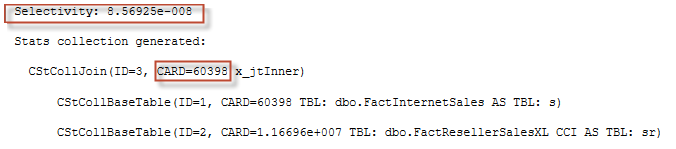
And the query plan:
和查询计划:
CSelCalcSimpleJoinWithDistinctCounts on Unique Key and Multicolumn Statistics
有关唯一键和多列统计信息的CSelCalcSimpleJoinWithDistinctCounts
The more interesting case is when SQL Server uses multicolumn statistics for the estimation, but there is no unique constraint. To look at this example, let’s compile the query similar to the previous one, but join FactInternetSales with the table FactInternetSalesReason. The table FactInternetSalesReason has a primary key on three columns (SalesOrderNumber, SalesOrderLineNumber, SalesReasonKey), so it also has multi-column statistics, but the combination (SalesOrderNumber, SalesOrderLineNumber) is not unique in that table.
更有趣的情况是SQL Server使用多列统计信息进行估计,但是没有唯一约束。 为了看这个例子,让我们编译与上一个查询类似的查询,但是将FactInternetSales与表FactInternetSalesReason连接起来。 表FactInternetSalesReason在三列(SalesOrderNumber,SalesOrderLineNumber,SalesReasonKey)上具有主键,因此它也具有多列统计信息,但是组合(SalesOrderNumber,SalesOrderLineNumber)在该表中不是唯一的。
select *
from
	dbo.FactInternetSales s
	join dbo.FactInternetSalesReason sr on
		s.SalesOrderNumber = sr.SalesOrderNumber and
		s.SalesOrderLineNumber = sr.SalesOrderLineNumber
option (querytraceon 3604, querytraceon 2363)
Let’s look at the selectivity computation plan:
让我们看一下选择性计算计划:
Parent calculator is still the same Simple Join On Distinct Counts, one sub-calculator is also the same, but the second sub-calculator is different, it is CDVCPlanLeaf with one multi-column stats available.
父计算器仍然是相同的,即“不同计数上的简单联接”,一个子计算器也相同,但是第二个子计算器却不同,它是CDVCPlanLeaf,具有一个多列统计信息。
We’ll get the density from the first table and the second table multi-column statistics for the join column combination:
我们将从联接列组合的第一个表和第二个表多列统计信息中获得密度:
dbcc show_statistics (FactInternetSales, PK_FactInternetSales_SalesOrderNumber_SalesOrderLineNumber) with density_vector;
dbcc show_statistics (FactInternetSalesReason, PK_FactInternetSalesReason_SalesOrderNumber_SalesOrderLineNumber_SalesReasonKey) with density_vector;
And get the minimum of two:
并获得至少两个:
This time it will be the density from FactInternetSales – 1.655684E-05. This is picked as a join predicate selectivity, and now multiply base cardinalities of those tables by this selectivity.
这次将是FactInternetSales – 1.655684E-05的密度。 选择它作为联接谓词的选择性,现在将这些表的基数基数乘以该选择性。
select 60398. * 64515. * 1.655684E-05 -- 64515.0014399748
Let’s check with the results from SQL Server.
让我们检查一下SQL Server的结果。
The query plan will show you also 64515 rows estimate in the join operator, however, I’ll omit the plan picture for brevity.
查询计划还将在联接运算符中向您显示64515行估计,但是,为简洁起见,我将省略计划图片。
CSelCalcSimpleJoinWithDistinctCounts on Single Column Statistics
CSelCalcSimpleJoinWithDistinctCounts单列统计
Finally let’s move on to the most common scenario, when there are no multi-column statistics, but there are single column statistics. Let’s compile the query (please don’t run this query, as it produces a huge result set):
最后,让我们继续进行最常见的情况,即没有多列统计信息,但是只有单列统计信息。 让我们编译查询(请不要运行此查询,因为它会产生巨大的结果集):
select *
from
	dbo.FactInternetSales si
	join dbo.FactResellerSales sr on
		si.CurrencyKey = sr.CurrencyKey and
		si.SalesTerritoryKey = sr.SalesTerritoryKey
option (querytraceon 3604, querytraceon 2363)
Again, we are joining FactInternetSales table, but this time with FactResellerSales table and on different columns: CurrencyKey and SalesTerritoryKey. Those columns have their own statistics and no multi-column stats. In that case SQL Server does more complicated mathematics, however, not too complex. In the SSMS message tab we may observe the plan for computation:
同样,我们将加入FactInternetSales表,但这一次是FactResellerSales表,并在不同的列上:CurrencyKey和SalesTerritoryKey。 这些列具有自己的统计信息,没有多列统计信息。 在那种情况下,SQL Server会执行更复杂的数学运算,但是并不太复杂。 在SSMS消息选项卡中,我们可以观察计算计划:
This time both sub-calculators are CDVCPlanLeaf and both of them are going to use 2 single-column statistics. SQL Server should somehow combine those statistics to get some common selectivity for the multi-column predicate. The next part of the output shows some computation details.
这次,两个子计算器均为CDVCPlanLeaf,并且它们都将使用2个单列统计信息。 SQL Server应该以某种方式组合这些统计信息以获得对多列谓词的一些通用选择性。 输出的下一部分显示了一些计算细节。
We’ll start with the first table FactInternetSales and the TF output related to it:
我们将从第一个表FactInternetSales及其相关的TF输出开始:
Two histograms (and in fact not only histograms, but the density vectors also) loaded for two columns, those statistics have ids 2 and 9 (# 1). Let’s query sys.stats to find them and look into.
为两列加载两个直方图(实际上不仅是直方图,还包括密度矢量),这些统计信息的ID为2和9(#1)。 让我们查询sys.stats来查找它们并进行调查。
select * from sys.stats where object_id = object_id('[dbo].[FactInternetSales]') and stats_id in (2,9)
dbcc show_statistics (FactInternetSales, _WA_Sys_00000007_276EDEB3) with density_vector;
dbcc show_statistics (FactInternetSales, _WA_Sys_00000008_276EDEB3) with density_vector;
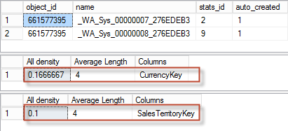
We see two densities for the two columns. The density is a measure of how many distinct values there are in the column, the formula is: density = 1/distinct_count. So to find distinct_count we use distinct_count = 1/density.
我们在两列中看到两种密度。 密度是衡量该列中有多少个不同值的度量,公式为:密度= 1 / distinct_count。 因此,要找到distinct_count,我们使用distinct_count = 1 / density。
It will be:
这将是:
select 1./0.1666667 -- 5.99999880 ~ 6
select 1./0.1 -- 10.000000
This is what we see in the computation output # 2.
这是我们在计算输出2中看到的。
Now SQL Server uses independency assumption, if we have 6 different CurrencyKeys and 10 different SalesTerritoryKeys, then how many unique pairs we may potentially have? It’s 6*10 = 60 unique pairs. So the combined distinct count is 60, as we can see in the output # 3.
现在,SQL Server使用独立性假设,如果我们有6个不同的CurrencyKeys和10个不同的SalesTerritoryKeys,那么我们可能有多少个唯一对? 它是6 * 10 = 60个唯一对。 因此,合并的非重复计数为60,正如我们在输出#3中看到的那样。
The similar math is then done for the second table, I will omit the computation, just show the result.
然后为第二张表完成类似的数学运算,我将省略计算,仅显示结果。
So far we have: 60 distinct values for the first table and 50 distinct values for the second one. Now we’ll get the densities using the formula described above density = 1/distinct_count.
到目前为止,我们有:第一个表有60个不同的值,第二个表有50个不同的值。 现在,我们将使用上面描述的公式来获得密度density = 1 / distinct_count 。
select 1E0/60. -- 0.0166666666666667
select 1E0/50. -- 0.02
Again, like we have done before, pick the minimum one: 0.0166666666666667 or rounded up to 7 digits 0.1666667. This will be the join predicate selectivity.
再次,就像我们之前所做的那样,选择最小的一个:0.0166666666666667或四舍五入为0.1666667的7位数字。 这将是连接谓词的选择性。
Now get the join cardinality by multiplying it with table cardinalities:
现在通过将其与表基数相乘来获得连接基数:
select 0.0166666666666667 * 60398. * 60855. -- 61258671.5000001225173430
If we round up 61258671.5000001225173430 it will be 61258700.
如果我们将61258671.5000001225173430舍入,则为61258700。
Now let’s check with SQL Server.
现在让我们检查一下SQL Server。
And in the query plan:
并在查询计划中:
You see that the selectivity and rounded cardinality match with what we have calculated manually. Now move on to the next example.
您会看到选择性和四舍五入的基数与我们手动计算的结果相匹配。 现在转到下一个示例。
CSelCalcSimpleJoin
CSelCalcSimpleJoin
It is possible to use distinct values when there is an equality predicate, because the distinct count tells us about how many unique discrete values are in the column and we may somehow combine the distinct count to model a join. If there is inequality predicate there is no more discrete values, we are talking about the intervals. In that case SQL Server uses calculator CSelCalcSimpleJoin.
当存在相等谓词时,可以使用不同的值,因为不同的数量会告诉我们该列中有多少个唯一的离散值,并且我们可能会以某种方式组合不同的数量来对联接进行建模。 如果存在不等式谓词,则不再有离散值,我们在谈论区间。 在这种情况下,SQL Server使用计算器CSelCalcSimpleJoin。
The algorithm used for a simple join respects different cases, but we will stop at the simplest one. The empirical formula for this case is: join_predicate_selectivity = max(1/card1; 1/card2), where card1 and card2 is a cardinality of the joining tables.
用于简单联接的算法适用于不同情况,但我们将在最简单的情况下停止。 这种情况的经验公式为:join_predicate_selectivity = max(1 / card1; 1 / card2),其中card1和card2是联接表的基数。
To demonstrate the example, we will take the query from the previous part and replace equality comparison with an inequality.
为了演示该示例,我们将从上一部分中获取查询,并将等式比较替换为不等式。
select *
from
	dbo.FactInternetSales s
	join dbo.FactResellerSalesXL_CCI sr on
		s.SalesOrderNumber = sr.SalesOrderNumber and
		s.SalesOrderLineNumber > sr.SalesOrderLineNumber
option (querytraceon 3604, querytraceon 2363)
The plan for computation on the message tab is:
消息选项卡上的计算计划是:
Not very informative, though you may notice a few interesting things.
虽然您可能会注意到一些有趣的事情,但它的信息量不是很多。
First of all, the new calculator CSelCalcSimpleJoin is used instead of CSelCalcSimpleJoinOnDistinctCounts. The second is the selectivity, which is rounded maximum of: max(1/Cardinality of FactInternetSales; 1/Cardinality of FactResellerSalesXL_CCI).
首先,使用新的计算器CSelCalcSimpleJoin代替CSelCalcSimpleJoinOnDistinctCounts。 第二个是选择性,取整后的最大值取整:max(1 / FactInternetSales的基数; 1 / FactResellerSalesXL_CCI的基数)。
select max(sel) from (values (1E+0/60398E+0), (1E+0/11669600E+0)) tbl(sel) -- 1.65568396304513E-05 ~ 1.65568E-05
The join cardinality is estimated as usual by multiplying base cardinalities with the join predicate selectivity, with obviously gives us 11669600:
通常,通过将基数基数与连接谓词选择性相乘来估算连接基数,显然得出11669600:
select 1.65568396304513E-05 * 60398E+0 * 11669600E+0 – 11669600
We may observe this estimation in the query plan:
我们可能会在查询计划中观察到这种估计:
If the cardinality of the FactResellerSalesXL_CCI was less than cardinality of FactInternetSales, let’s say one row less 60398-1 = 60397, than the value 1/60397 would be picked. In that case the join cardinality would be 60398:
如果FactResellerSalesXL_CCI的基数小于FactInternetSales的基数,则可以说比60398-1 = 60397少一行,比值1/60397少。 在这种情况下,联接基数为60398:
select (1E+0/60397E+0)* (60397E+0) * (60398E+0) -- 60398
Let’s test this by tricking the optimizer with update statistics command with undocumented argument rowcount like this:
让我们通过使用update statistics命令欺骗优化器并使用未记录的参数rowcount进行测试,如下所示:
-- trick the optimizer
update statistics FactResellerSalesXL_CCI with rowcount = 60397;
go
-- compile
set showplan_xml on;
go
select *
from
	dbo.FactInternetSales s
	join dbo.FactResellerSalesXL_CCI sr on
		s.SalesOrderNumber = sr.SalesOrderNumber and
		s.SalesOrderLineNumber > sr.SalesOrderLineNumber
option (querytraceon 3604, querytraceon 2363)
go
set showplan_xml off;
go
-- return to original row count
update statistics FactResellerSalesXL_CCI with rowcount = 11669600;
If you switch to the message tab you will see that the join selectivity is now 1.65571e-005:
如果切换到消息选项卡,您将看到联接选择性现在为1.65571e-005:
Which is rounded value of:
四舍五入后的值:
select 1E0/60397E0 -- 1.65571137639287E-05
And the join cardinality is now 60398, as well as in the query plan:
现在,查询计划中的联接基数为60398:
We’ll now move on to the next calculator, new in SQL Server 2016 and CE 130.
现在,我们将继续使用SQL Server 2016和CE 130中的下一个计算器。
CSelCalcSimpleJoinWithUpperBound (new in 2016)
CSelCalcSimpleJoinWithUpperBound(2016年新增)
If we compile the last query under 120 compatibility level and 130 we will notice the estimation differences. I will add a TF 9453 to the second query, that restricts Batch execution mode and a misleading Bitmap Filter (misleading only in our demo purposes, as we need only join and no other operators). To be honest, we may add this TF to the first one query also, though it is not necessary. (Frankly speaking this TF is not needed at all, because it does not influence the estimate, however, I’d like to have a simple join plan for the demo).
如果我们在120兼容级别和130兼容级别下编译最后一个查询,我们将注意到估计差异。 我将在第二个查询中添加一个TF 9453,它限制了批处理执行模式和一个误导性的位图过滤器(仅出于演示目的而引起误解,因为我们仅需要联接而无需其他运算符)。 老实说,我们也可以将此TF添加到第一个查询中,尽管这不是必需的。 (坦白地说,完全不需要此TF,因为它不会影响估计,但是,我想为该演示制定一个简单的加入计划)。
Let’s run the script to observe the different estimates:
让我们运行脚本来观察不同的估计:
alter database [AdventureworksDW2016CTP3] set compatibility_level = 120;
go
set showplan_xml on;
go
select *
from
	dbo.FactInternetSales s
	join dbo.FactResellerSalesXL_CCI sr on
		s.SalesOrderNumber = sr.SalesOrderNumber and
		s.SalesOrderLineNumber > sr.SalesOrderLineNumber
option (querytraceon 3604, querytraceon 2363, querytraceon 9453);
go
set showplan_xml off;
go
alter database [AdventureworksDW2016CTP3] set compatibility_level = 130;
go
set showplan_xml on;
go
select *
from
	dbo.FactInternetSales s
	join dbo.FactResellerSalesXL_CCI sr on
		s.SalesOrderNumber = sr.SalesOrderNumber and
		s.SalesOrderLineNumber > sr.SalesOrderLineNumber
option (querytraceon 3604, querytraceon 2363, querytraceon 9453);
go
set showplan_xml off;
go
The estimates are very different:
估计差异很大:
Eleven million rows for the CE 120 and half a million for CE 130.
CE 120为一千一百万,CE 130为一百万。
If we inspect the TF output for the CE 130, we will see that it doesn’t use calculator CSelCalcSimpleJoin, but uses the new one CSelCalcSimpleJoinWithUpperBound.
如果我们检查CE 130的TF输出,我们将看到它不使用计算器CSelCalcSimpleJoin,而是使用新的CSelCalcSimpleJoinWithUpperBound。
You may also note that as a sub-calculator it uses already familiar to us calculator CSelCalcSimpleJoinWithDistinctCounts, described earlier, and this sub-calculator uses single column statistics.
您可能还注意到,作为子计算器,它使用了我们之前已经熟悉的计算器CSelCalcSimpleJoinWithDistinctCounts,并且该子计算器使用了单列统计信息。
If we look further, we will see that the statistics is loaded for the equality part of the join predicate on columns SalesOrderNumber for both tables.
如果进一步看,我们将看到两个表的SalesOrderNumber列上的连接谓词的相等部分均已加载统计信息。
Combined distinct counts could be found from the density vectors as we saw earlier in this post:
正如我们在本文前面所看到的,可以从密度向量中找到组合的不同计数:
dbcc show_statistics (FactInternetSales, PK_FactInternetSales_SalesOrderNumber_SalesOrderLineNumber) with density_vector;
dbcc show_statistics (FactResellerSalesXL_CCI, PK_FactResellerSalesXL_CCI_SalesOrderNumber_SalesOrderLineNumber) with density_vector;
So the distinct count would be:
因此,不同的计数将是:
select 1E0/3.61546E-05 -- 27658.9977485576
select 1E0/5.991565E-07 -- 1669013.02080508
Which equals to what we see in the output after round up. There is no need to combine distinct values here, because the equality part contains only one equality predicate (s.SalesOrderNumber = sr.SalesOrderNumber), but if we had condition like: join … on a1=a2 and b1=b2 and c1<c3, then we could combine distinct values for the part a1=a2 and b1=b2 to calculate its selectivity.
等于四舍五入后的输出结果。 这里不需要合并不同的值,因为相等部分仅包含一个相等谓词(s.SalesOrderNumber = sr.SalesOrderNumber),但是如果我们有这样的条件:在a1 = a2和b1 = b2上加入…且c1 <c3 ,那么我们可以组合部分a1 = a2和b1 = b2的不同值以计算其选择性。
In this case we will simply take the minimum of densities – 5.99157e-007 and multiply cardinalities with it:
在这种情况下,我们将简单地采用最小密度– 5.99157e-007并乘以基数:
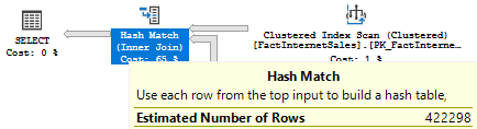
select 5.99157e-007 * 60398E0 * 11669600E0 -- 422298.136797826
This cardinality will be the upper boundary for the Simple Join estimation. If we look at the plan, we’ll see that this boundary is used as an estimate:
该基数将成为简单连接估计的上限。 如果看一下计划,我们将看到该边界被用作估计:
If we trick the optimizer with the script as we did before:
如果我们像以前一样用脚本欺骗优化器:
-- trick the optimizer
update statistics FactResellerSalesXL_CCI with rowcount = 60397; -- modified
go
-- compile
set showplan_xml on;
go
select *
from
	dbo.FactInternetSales s
	join dbo.FactResellerSalesXL_CCI sr on
		s.SalesOrderNumber = sr.SalesOrderNumber and
		s.SalesOrderLineNumber > sr.SalesOrderLineNumber
option (querytraceon 3604, querytraceon 2363, querytraceon 9453, maxdop 1)
go
set showplan_xml off;
go
-- return to original row count
update statistics FactResellerSalesXL_CCI with rowcount = 11669600;
We won’t get the estimate:
我们不会得到估计:
select 5.99157e-007 * 60398E0 * 60397E0 -- 2185.63965930094
Because this time the upper boundary is less than a simple join estimate (demonstrated earlier), so the last one will be picked:
因为这一次的上限小于一个简单的连接估计(前面已演示),所以将选择最后一个:
Finally I ran this query to get the actual number of rows:
最后,我运行此查询以获取实际的行数:
Both CE heavily overestimates. However, the 130 CE is closer to the truth.
两个CE都严重高估了。 但是,公元130年更加接近事实。
型号变化 (Model Variation)
There is a TF that forces the optimizer to use Simple Join algorithm even if a histogram is available. I will give you this one for the test and educational purposes. TF 9479 will force optimizer to use a simple join estimation algorithm, it may be CSelCalcSimpleJoinWithDistinctCounts, CSelCalcSimpleJoin or CSelCalcSimpleJoinWithUpperBound, depending on the compatibility level and predicate comparison type. You may use it for the test purposes and in the test enviroment only.
即使有直方图,也有一个TF强制优化器使用简单连接算法。 我会给您这个用于测试和教育目的。 TF 9479将强制优化器使用简单的联接估计算法,取决于兼容性级别和谓词比较类型,它可以是CSelCalcSimpleJoinWithDistinctCounts,CSelCalcSimpleJoin或CSelCalcSimpleJoinWithUpperBound。 您只能将其用于测试目的,并且只能在测试环境中使用。
摘要 (Summary)
There is a lot of information about join estimation algorithms over the internet, but very few about how SQL Server does it. This article showed some cases and demonstrated its maths and internals in calculating joins cardinality. This is by no means a comprehensive join estimation analysis article, but a short insight into this world. There are much more join algorithms, even if we look at the calculators: CSelCalcAscendingKeyJoin, CSelCalcFixedJoin, CSelCalcIndependentJoin, CSelCalcNegativeJoin, CSelCalcGuessComparisonJoin. And if we remember that one calculator can encapsulate several algorithms and SQL Server can even combine calculators – that is a really huge field of variants.
关于Internet上的联接估计算法的信息很多,但是关于SQL Server的工作方式的信息很少。 本文介绍了一些情况,并演示了其在计算联接基数时的数学和内部原理。 这绝不是一篇详尽的联接估计分析文章,而是对这个世界的简短了解。 即使我们看一下计算器,联接算法也会更多:CSelCalcAscendingKeyJoin,CSelCalcFixedJoin,CSelCalcIndependentJoin,CSelCalcNegativeJoin,CSelCalcGuessComparisonJoin。 而且,如果我们还记得一个计算器可以封装多种算法,而SQL Server甚至可以组合计算器,那将是一个很大的变体领域。
I think you now have an idea how the join estimation is done and how subtle differences about predicate types, count, comparison operators influence the estimates.
我认为您现在已经知道联接估计是如何完成的,以及谓词类型,计数,比较运算符之间的细微差异如何影响估计。
Thank you for reading!
感谢您的阅读!


 967
967

 被折叠的 条评论
为什么被折叠?
被折叠的 条评论
为什么被折叠?
 到【灌水乐园】发言


