sql 哈希匹配_SQL Server –哈希联接执行内部

sql 哈希匹配

Some time ago, on the 24HOP Russia I was talking about the Query Processor internals and joins. Despite I had three hours, I felt the lack of time, and something left behind, because it is a huge topic, if you try to cover it in different aspects in details. With the few next articles, I’ll try to describe some interesting parts of my talk in more details. I will start with Hash Join execution internals.

前段时间，在24HOP Russia上，我在谈论查询处理器的内部和联接。 尽管我花了三个小时，但我仍然感到时间紧缺，还有一些遗漏，因为如果您尝试在各个方面进行详细介绍，这是一个巨大的话题。 在接下来的几篇文章中，我将尝试更详细地描述我的演讲中一些有趣的部分。 我将从哈希联接执行内部开始。

The Hash Match algorithm is one of the three available algorithms for joining two tables together. However, it is not only about joining. You may observe a complete list of the logical operations that Hash Match supports in the documentation:

哈希匹配算法是将两个表连接在一起的三种可用算法之一。 但是，这不仅与加入有关。 您可能会在文档中观察到哈希匹配支持的逻辑操作的完整列表：

There are quite interesting logical operators implemented by Hash Match, like Partial Aggregate, or even more exotic Flow Distinct. Still, all that is very interesting, the focus of this post is on the Hash Match execution internals in the inner join row mode for regular tables (not in-memory tables).

Hash Match实现了一些非常有趣的逻辑运算符，例如Partial Aggregate，甚至更奇特的Flow Distinct 。 尽管如此，所有有趣的事情还是，本文的重点是常规表（而非内存表）的内部联接行模式下的哈希匹配执行内部。

内存算法 (In memory Algorithm)

The simplified process as a whole might be illustrated as follows.

整个简化的过程可能如下所示。

Hash Match in the join mode consumes two inputs, as we are joining two tables. The main idea is to build the hash table using the first “build” input, and then apply the same approach hash the second “probe” input to see if there will be matches of hashed values.

在联接模式下，哈希匹配消耗两个输入，因为我们正在联接两个表。 主要思想是使用第一个“构建”输入构建哈希表，然后对第二个“探针”输入应用相同的方法对哈希进行哈希，以查看是否存在匹配的哈希值。

Query Processor (QP) is doing many efforts while building the plan to choose the correct join order. From the Hash Match prospective, it means that QP should choose what table is on the Build side and what is on the Probe side. The Build size should be smaller as it will be stored in memory when building a hash table.

查询处理器（QP）在制定计划以选择正确的连接顺序时正在做很多工作。 从哈希匹配的角度来看，这意味着QP应该选择在Build端是什么表，在Probe端是什么表。 构建大小应该较小，因为在构建哈希表时它将存储在内存中。

Building a hash table begins with hashing join key values of the build table and placing them to one or another bucket depending on the hash value. Then QP starts processing the probe side, it applies the same hash function to the probe values, determining the bucket and compares the values inside of the bucket. If there is a match – the row is returned.

构建哈希表时，首先需要对哈希表的连接键值进行哈希处理，然后根据哈希值将其放置到一个或另一个存储桶中。 然后，QP开始处理探测端，它将相同的哈希函数应用于探测值，确定存储桶并比较存储桶内部的值。 如果存在匹配项，则返回该行。

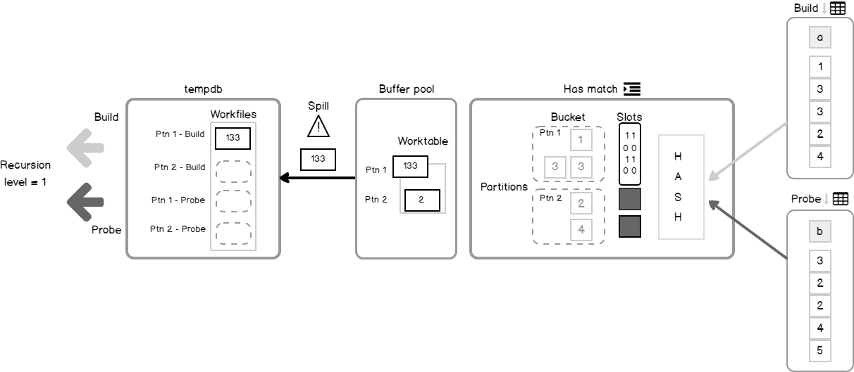
That would be the whole story if we had infinite memory, but in the real world, it is not true. More to the point, SQL Server allocates memory to the query before the execution starts and does not change it during the execution. That means that if the allocated memory amount is much less than the data size came during the execution, a Hash Match should be able to partition the joining data, and process it in portions that fit allocated memory, while the rest of the data is spilled to the disk waiting to be processed. Here is where the dancing begins.

如果我们拥有无限的记忆，那将是完整的故事，但是在现实世界中，事实并非如此。 更重要的是，SQL Server在执行开始之前为查询分配内存，并且在执行期间不更改内存。 这意味着，如果分配的内存量远小于执行期间的数据大小，则哈希匹配应该能够对联接数据进行分区，并在适合分配的内存的部分中对其进行处理，而其余数据则被溢出。到等待处理的磁盘。 舞蹈在这里开始。

通用算法 (General Algorithm)

A couple of pictures to illustrate the algorithm. The first one depicts the structures.

两张图片说明了该算法。 第一个描述了结构。

Build