sql2018 ssas_在SQL Server Analysis Services（SSAS）2016中使用多对多关系

最新推荐文章于 2021-04-07 20:19:52 发布

culuo4781

最新推荐文章于 2021-04-07 20:19:52 发布

阅读量433

点赞数

文章标签：机器学习数据分析人工智能大数据数据库

原文链接：https://www.sqlshack.com/using-many-many-relationships-sql-server-analysis-services-ssas-2016/

版权

sql2018 ssas

The Multidimensional Cube option of Analysis Services has handled many-to-many relationships with ease for many versions before 2016. The Tabular had a work around using DAX formulas until the release of SQL Server 2016. There are still some limitations to many-to many in Tabular but of course, there are some “tricks” to overcome the limitations. But, the many-to-many relationship will be in businesses data for many years to come. A solution has to be provided when it comes to Analysis Service databases.

Analysis Services的多维多维数据集选项在2016年之前已轻松处理了许多版本的多对多关系。在SQL Server 2016发行之前，表格已解决了使用DAX公式的问题。多对多仍然存在一些局限性在表格中，但是当然有一些“技巧”可以克服这些限制。但是，在未来许多年中，多对多关系将存在于业务数据中。当涉及Analysis Service数据库时，必须提供一个解决方案。

Before going to the development and support of many-to-many in Analysis Services, the ETL of a reporting application has to format the data in tables conducive to supporting this option. This might be referred to as a bridge table. The data in the transaction table is “bridged” to the many possible supporting categories. The Adventure Works DW data provides a great example with many Sales Reasons related to many Internet Sales Line Items.

在进行Analysis Services中的多对多开发和支持之前，报表应用程序的ETL必须将数据格式化为有利于支持此选项的表。这可以称为桥表。交易表中的数据被“桥接”到许多可能的支持类别。 Adventure Works DW数据提供了一个很好的示例，其中包含与许多Internet销售订单项相关的许多销售原因。

Figure 1 shows an example of the design of these tables.

图1显示了这些表的设计示例。

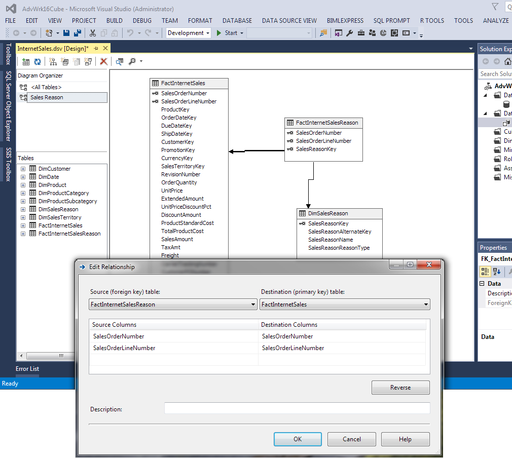
The Edit Relationship in Figure 1 shows in a cube the relationship between 2 tables with multiple columns – SalesOrderNumber (Order Number) and SaleOrderLineNumber (Order Line Number). This bridge table, FactInternetSalesReason, bridges the Sales Reasons from the DimSalesReason dimension table to the FactinternetSales fact table by these 2 columns. The FactInternetSalesReason table can have multiple entries for the same Order Number plus Order Line Number. The example in the table below shows 2 different Sales Order Number with 3 different Sales Reason.

图1中的Edit Relationship在一个多维数据集中显示了具有多列的2个表之间的关系– SalesOrderNumber（订单号）和SaleOrderLineNumber（订单线号）。该桥接表FactInternetSalesReason通过这2列将销售原因从DimSalesReason维度表桥接到FactinternetSales事实表。 FactInternetSalesReason表可以为同一订单号加上订单行号包含多个条目。下表中的示例显示了2个不同的销售订单编号和3个不同的销售原因。

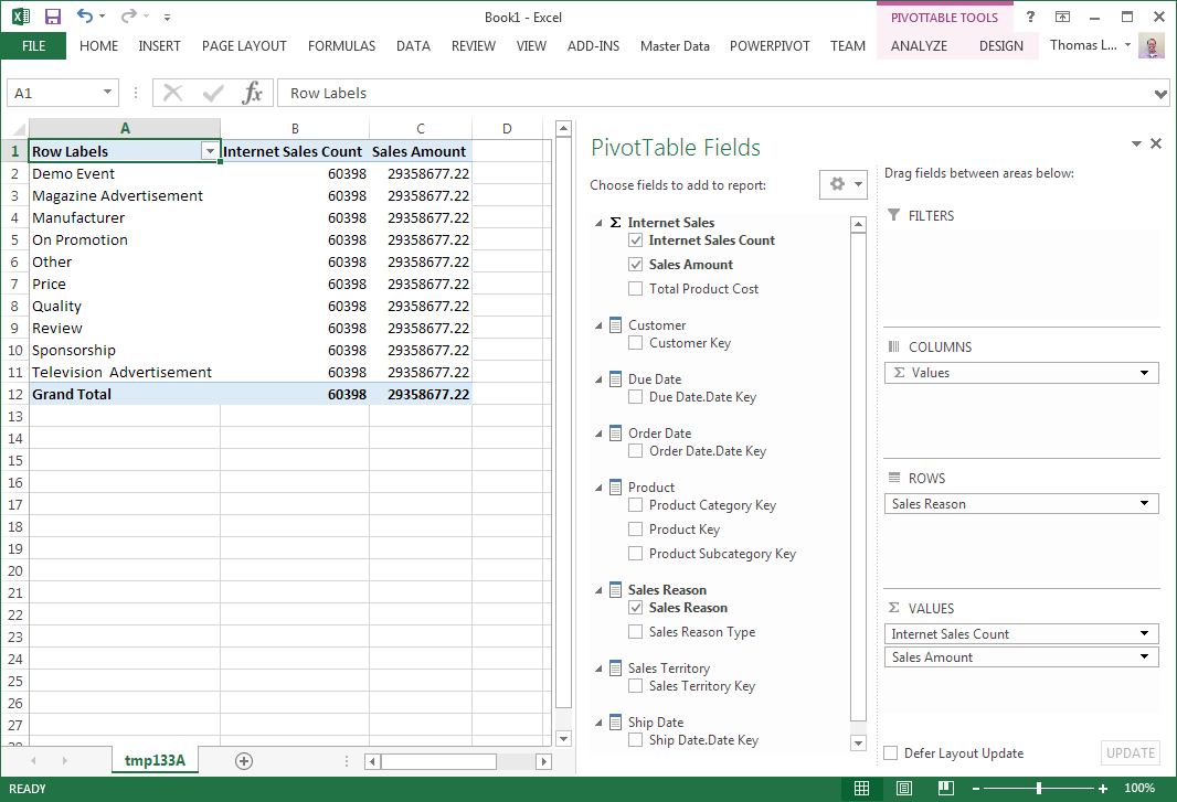
Figure 2 shows the Analyze in Excel when there is no relationship between Sales Reason and Internet Sales for the cube. This is the same output initially received with Tabular as well. Many-to-many relationships are not automatically assigned with building a cube or tabular model through the wizards. There is more work to be done after the wizard completes. The Sales Count and Sale Amount measures are summed on all rows rather than the Sales Reason slicer used in Figure 2.

图2显示了多维数据集的“销售原因”与“ Internet销售”之间没有关系时的Excel分析。这也是最初与Tabular一起接收的输出。通过向导构建多维数据集或表格模型不会自动分配多对多关系。向导完成后，还有更多工作要做。 “销售计数”和“销售金额”度量是所有行的总和，而不是图2中使用的“销售原因”切片器。

The relationship is not a regular relationship for the Dimension Relationship in the Cube. But before setting the relationship, the Sales Reason (DimSalesReason table) and Fact Internet Sales (FactInternetSales table) dimensions need to be created plus a Measure Group for fact table FactInternetSalesReason. The measure can be a count of rows and hidden through the Visible property of the measure. Once these are created, the many-to-many relationship can be created in the Cube Dimension Relationship between the Sales Reason Dimension and Internet Sales Measure group like in Figure 3.

对于多维数据集中的尺寸关系，该关系不是常规关系。但是在设置关系之前，需要创建销售原因（DimSalesReason表）和事实Internet销售（FactInternetSales表）维度，以及事实表FactInternetSalesReason的度量值组。度量可以是行的计数，并且可以通过度量的Visible属性隐藏。一旦创建了这些，就可以在“销售原因”维度和“ Internet销售度量”组之间的“多维数据集”维度关系中创建多对多关系，如图3所示。

Below the Sales Reason relationship to Internet Sales measure group is a Fact Relationship between Fact Internet Sales dimension and Internet Sales measure group. Fact tables can be dimensions in Analysis Service and contain attributes like PO Number or Freight Company. It can also be created for this relationship and made Visible = False in the cube. The Sales Reason and Fact Internet Sales dimensions are related to new measure group by regular relationships.

“与Internet销售”度量标准的“销售原因”关系下方是“事实Internet销售”维度和“ Internet销售”度量值组之间的“事实关系”。事实表可以是Analysis Service中的维度，并包含诸如PO Number或Freight Company之类的属性。也可以为此关系创建它，并在多维数据集中使Visible = False。销售原因和事实互联网销售维度通过常规关系与新的度量值组相关。

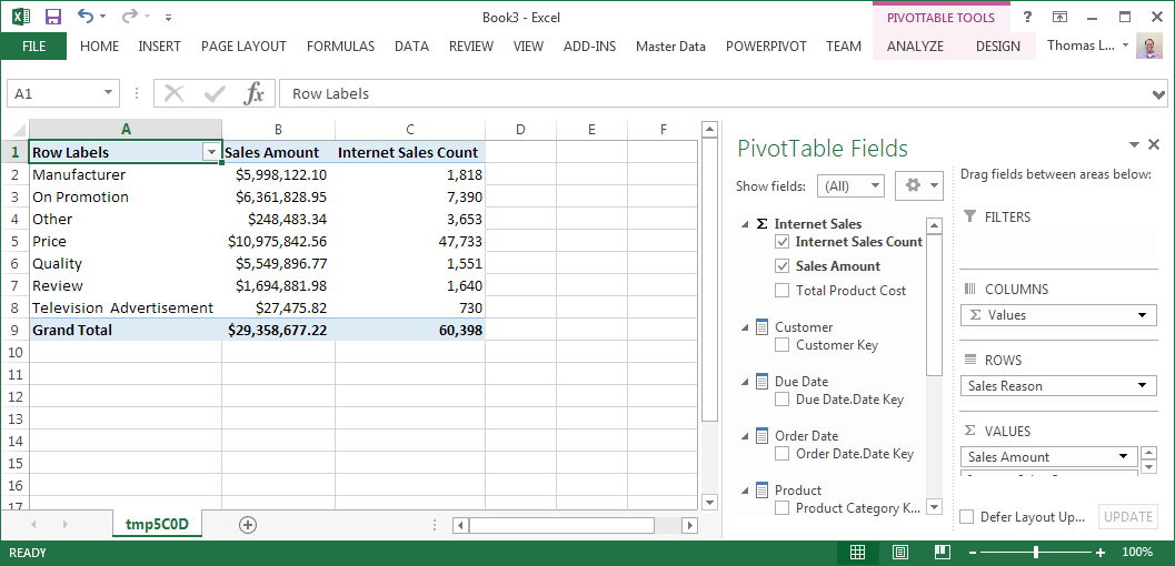
Figure 4 now shows correct counts and dollar amounts while Analyzing in Excel. The Sales Amount total as Grand Total is the correct total of all sales filtered. But the Sum of the Sales Reason totals in the pivot table will be more than the grand total because of sales having multiple sales reasons. Training end users about this variation are important.

现在，图4显示了在Excel中进行分析时的正确计数和美元金额。作为总计的“销售总额”是所有已过滤销售的正确总数。但是，由于销售有多个销售原因，因此数据透视表中的“销售原因之和”总数将大于总计。对最终用户进行有关此变化的培训非常重要。

The Tabular Model of Analysis Services uses a new feature in SQL Server 2016 called bi-directional filtering. Bi-directional filtering is used for many-to-many. The creation of bi-directional filtering is for filtering through one table, say a fact table, to an aggregation in a dimension table. Some might go activate this on every relationship, but Microsoft warns not to do this. Just implement where needed.

Analysis Services的表格模型使用SQL Server 2016中的一项新功能，即双向筛选。双向过滤用于多对多。双向过滤的创建是为了将一个表（例如事实表）过滤到维表中的聚合。某些人可能会在每种关系上都激活它，但是Microsoft警告不要这样做。只需在需要的地方实施即可。

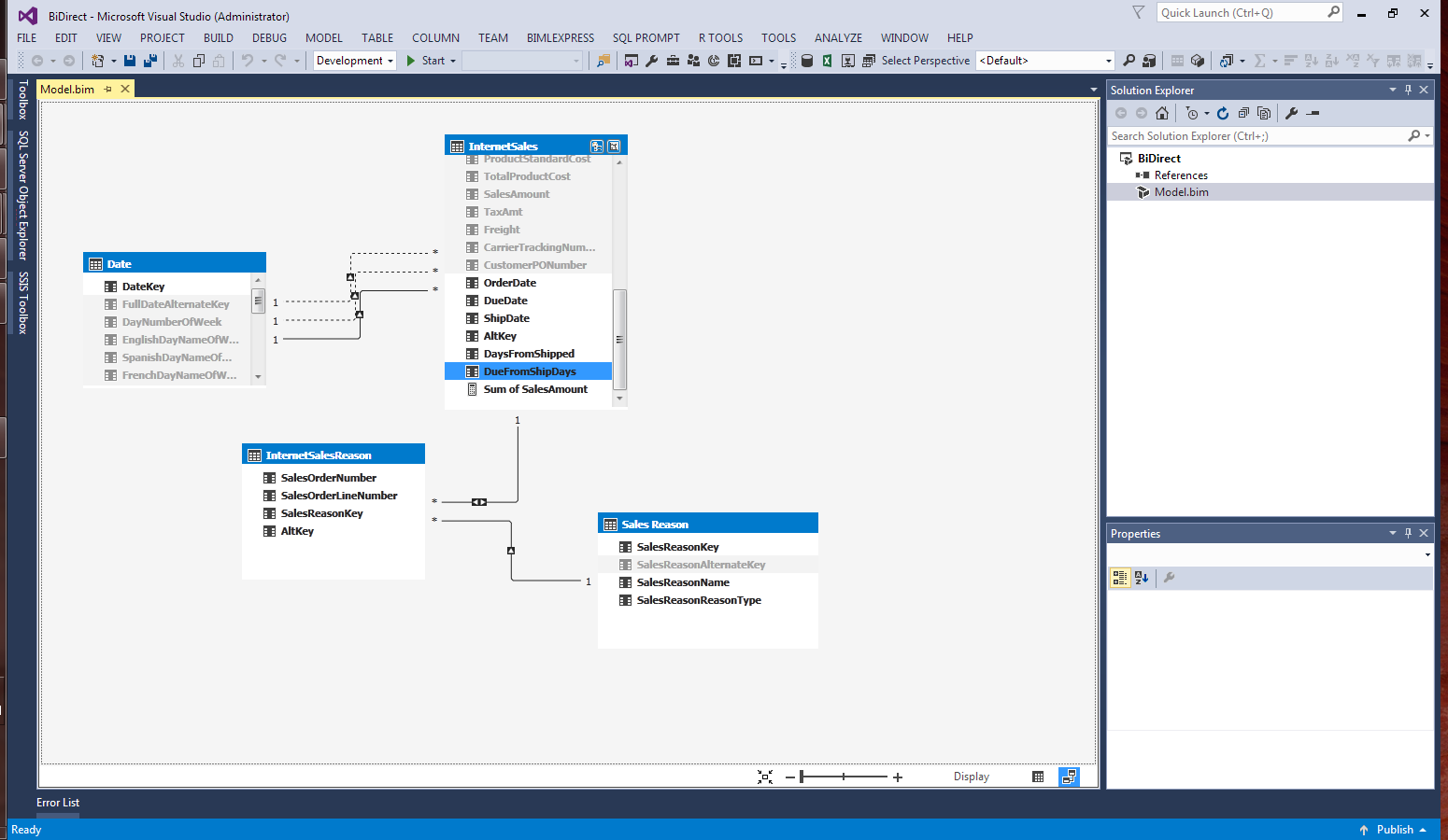
The only many-to-many this will work with is a 3 table many-to-many. Figure 5 shows the Fact Internet Sales, Fact Internet Sales Reason and Sales Reason in a Tabular Model. Do not use this when more than 3 tables are involved in a many-to-many relationship.

唯一可以使用的多对多表是3对多表。图5以表格模型显示了事实互联网销售，事实互联网销售原因和销售原因。当多对多关系涉及三个以上的表时，请勿使用此选项。

What cannot be seen in this example is the columns used to relate InternetSalesReason to InternetSales. The relationships in the Tabular Model (and in Power BI) can only be one column. So, this example uses a calculated column in the InternetSales and InternetSalesReason table. Figure 6 shows this relationship.

在此示例中看不到用于将InternetSalesReason与InternetSales相关联的列。表格模型（和Power BI）中的关系只能是一列。因此，本示例使用InternetSales和InternetSalesReason表中的计算列。图6显示了这种关系。

Also, the Filter Direction drop-down shows “To Both Table” instead of to the many sides of a relationship. This is the bi-directional filtering option. The column used to relate the 2 tables is called AltKey. Figure 7 shows the calculated column in the InternetSalesReason table.

此外，“过滤器方向”下拉列表显示“到两个表”，而不是关系的多个方面。这是双向过滤选项。用于关联这两个表的列称为AltKey。图7显示了InternetSalesReason表中的计算列。

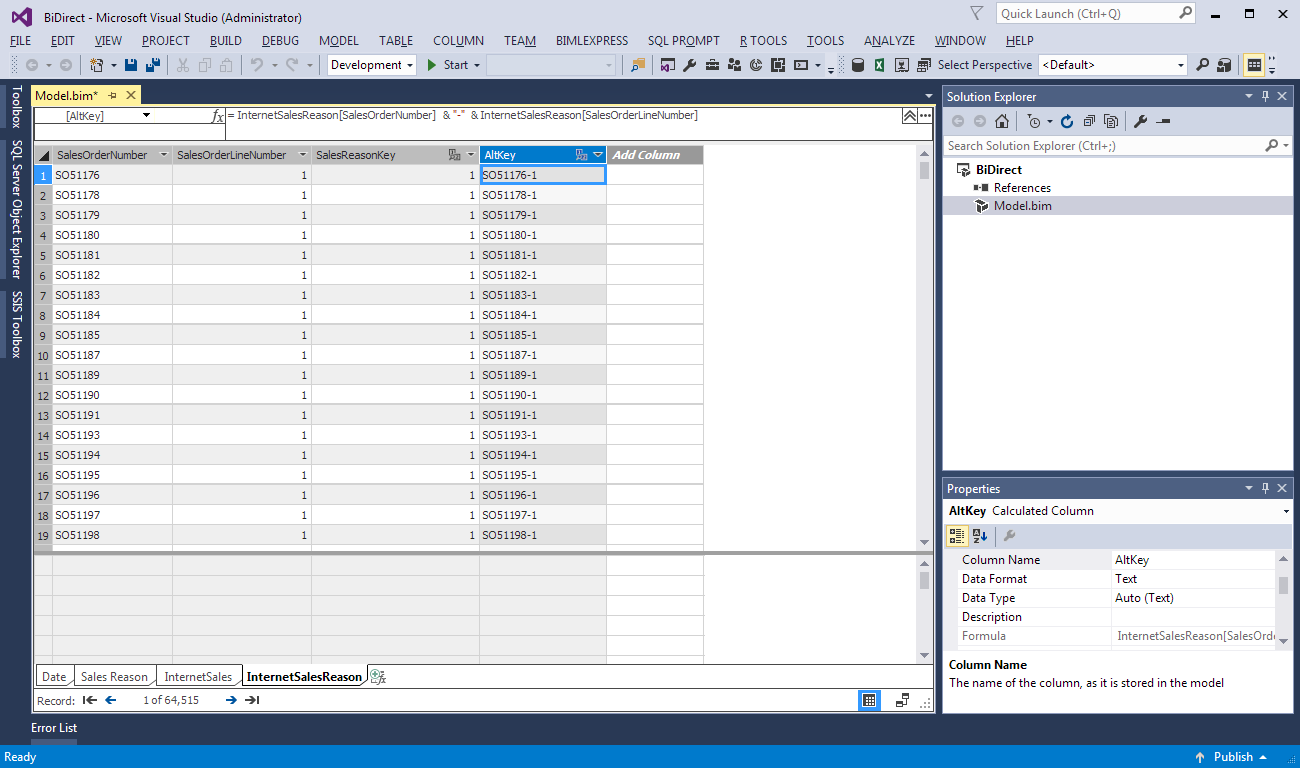
The AltKey computed column uses this logic –InternetSalesReason [SalesOrderNumber] & “-” & InternetSalesReason [SalesOrderLineNumber]. The SalesOrderNumber is concatenated with the SalesOrderLineNumber with a dash between the 2 values. This column creates an alternate key for the tables. Since it is created in both InternetSales and InternetSalesReason, they can be used to join the 2 fact tables. Remember, the InternetSalesReason table is the bridge table between DimSalesReason and FactInternetSales.

AltKey计算列使用此逻辑– InternetSalesReason [SalesOrderNumber]和“-”和InternetSalesReason [SalesOrderLineNumber]。 SalesOrderNumber与SalesOrderLineNumber串联在一起，两个值之间用短划线表示。此列为表创建备用键。由于它是在InternetSales和InternetSalesReason中创建的，因此可以将它们用于连接2个事实表。请记住，InternetSalesReason表是DimSalesReason和FactInternetSales之间的桥梁表。

The Bi-Directional filtering can be used in another way. Says the end user wants to view a count of distinct products associated with the Sales list by a particular year. A normal many-to-one relationship will not be able to show that. Figure 8 shows the normal DimProduct relationship to InternetSales.

双向过滤可以以其他方式使用。表示最终用户希望按特定年份查看与“销售”列表关联的不同产品的数量。正常的多对一关系将无法证明这一点。图8显示了正常的DimProduct与InternetSales的关系。

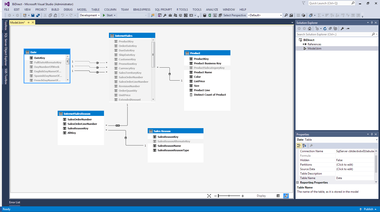
Figure 9 shows the Distinct Count of products with a filter on year for Internet Sales.

图9显示了按互联网销售情况过滤的产品的非重复计数。

The Distinct Count is the same for all years, even years without any sales. Changing the relationship in the diagram view of the Tabular Model will solve this problem like Figure 10.

所有年份（甚至没有任何销售的年份）的“不重复计数”都是相同的。在表格模型的图表视图中更改关系将解决如图10所示的问题。

Figure 11 shows the Analyze in Excel results from using bi-directional filtering on the Production table relationship with the InternetSales table.

图11显示了在Production表和InternetSales表之间使用双向过滤后在Excel中进行分析的结果。

Analysis Services has been able to handle business logic like this in MDX and DAX. But users are more interested in these logical business rules to be implemented in the database. The Tabular Model is starting to look more and more like the Multidimensional Cube with the end result, not in the method of obtaining the result. Luckily there are plenty of users in the Microsoft Data Technology community willing to show how this works. Watch the new stuff coming in SQL Server 2017 and stay up with the changes.

Analysis Services能够处理MDX和DAX中的这种业务逻辑。但是用户对这些要在数据库中实现的逻辑业务规则更感兴趣。表格模型越来越看起来像具有多维结果的多维数据集，而不是获得结果的方法。幸运的是，Microsoft数据技术社区中有很多用户愿意展示其工作原理。观看SQL Server 2017中的新内容，并及时掌握变化。