


kaggle 入门
Founded in 2010, Kaggle is a Data Science platform where users can share, collaborate, and compete. One key feature of Kaggle is “Competitions”, which offers users the ability to practice on real world data and to test their skills with, and against, an international community.
Kaggle成立于2010年,是一个数据科学平台,用户可以在其中共享,协作和竞争。 Kaggle的一项主要功能是“竞争”,它为用户提供了在现实世界数据上进行练习以及与国际社会进行对抗的能力,以测试其技能。
This guide will teach you how to approach and enter a Kaggle competition, including exploring the data, creating and engineering features, building models, and submitting predictions. We’ll use Python 3 and Jupyter Notebook.
本指南将教您如何进入和参加Kaggle竞赛,包括探索数据,创建和工程特征,构建模型以及提交预测。 我们将使用Python 3和Jupyter Notebook 。
竞赛 (The Competition)
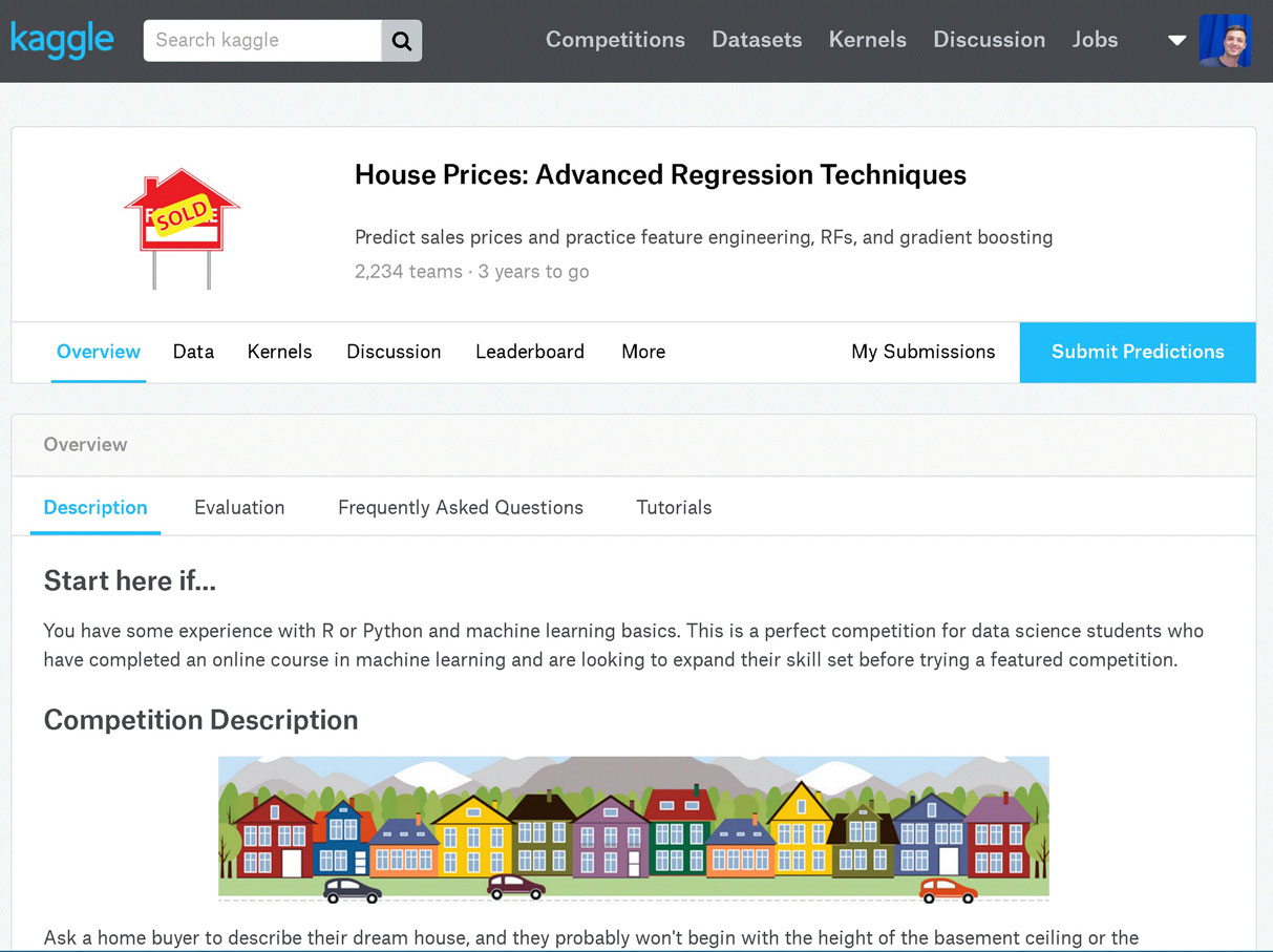
We’ll work through the House Prices: Advanced Regression Techniques competition.
我们将完成“ 房价:高级回归技术”竞赛。
We’ll follow these steps to a successful Kaggle Competition submission:
我们将按照以下步骤成功提交Kaggle竞赛:
- Acquire the data
- Explore the data
- Engineer and transform the features and the target variable
- Build a model
- Make and submit predictions
- 采集数据
- 探索数据
- 设计并转换特征和目标变量
- 建立模型
- 做出并提交预测
步骤1:获取数据并创建环境 (Step 1: Acquire the data and create our environment)
We need to acquire the data for the competition. The descriptions of the features and some other helpful information are contained in a file with an obvious name, data_description.txt.
我们需要获取比赛数据 。 这些功能的描述和其他一些有用的信息包含在一个文件中,文件的名称很明显data_description.txt 。
Download the data and save it into a folder where you’ll keep everything you need for the competition.
下载数据并将其保存到文件夹中,以保存比赛所需的一切。
We will first look at the train.csv data. After we’ve trained a model, we’ll make predictions using the test.csv data.
我们将首先查看train.csv数据。 训练模型后,我们将使用test.csv数据进行预测。
First, import Pandas, a fantastic library for working with data in Python. Next we’ll import Numpy.
首先,导入Pandas ,这是一个使用Python处理数据的绝佳库。 接下来,我们将导入Numpy 。
import import pandas pandas as as pd
pd
import import numpy numpy as as np
np
We can use Pandas to read in csv files. The pd.read_csv() method creates a DataFrame from a csv file.
我们可以使用Pandas读取csv文件。 pd.read_csv()方法从csv文件创建一个DataFrame。
Let’s check out the size of the data.
让我们检查一下数据的大小。
print print (( "Train data shape:""Train data shape:" , , traintrain .. shapeshape )
)
print print (( "Test data shape:""Test data shape:" , , testtest .. shapeshape )
)
Train data shape: (1460, 81)
Test data shape: (1459, 80)
We see that test has only 80 columns, while train has 81. This is due to, of course, the fact that the test data do not include the final sale price information!
我们看到test只有80列,而train只有81列。这当然是由于测试数据不包含最终售价信息!
Next, we’ll look at a few rows using the DataFrame.head() method.
接下来,我们将使用DataFrame.head()方法查看几行。
| Id | ID | MSSubClass | MSSubClass | MSZoning | 分区 | LotFrontage | LotFrontage | LotArea | LotArea | Street | 街 | Alley | 胡同 | LotShape | LotShape | LandContour | 陆地轮廓 | Utilities | 实用工具 | LotConfig | LotConfig | LandSlope | 土地坡度 | Neighborhood | 邻里 | Condition1 | 条件1 | Condition2 | 条件2 | BldgType | BldgType | HouseStyle | 家庭风格 | OverallQual | 综合素质 | OverallCond | 综合条件 | YearBuilt | 建立年份 | YearRemodAdd | YearRemodAdd | RoofStyle | 屋顶风格 | RoofMatl | 屋顶材料 | Exterior1st | 外观1 | Exterior2nd | 外观第二 | MasVnrType | MasVnrType | MasVnrArea | MasVnrArea | ExterQual | 扩展质量 | ExterCond | ExterCond | Foundation | 基础 | BsmtQual | 质量标准 | BsmtCond | BsmtCond | BsmtExposure | BsmtExposure | BsmtFinType1 | BsmtFinType1 | BsmtFinSF1 | BsmtFinSF1 | BsmtFinType2 | BsmtFinType2 | BsmtFinSF2 | BsmtFinSF2 | BsmtUnfSF | BsmtUnfSF | TotalBsmtSF | TotalBsmtSF | Heating | 加热 | HeatingQC | 加热QC | CentralAir | 中央航空 | Electrical | 电的 | 1stFlrSF | 1stFlrSF | 2ndFlrSF | 2ndFlrSF | LowQualFinSF | 低质量金融 | GrLivArea | GrLivArea | BsmtFullBath | BsmtFullBath | BsmtHalfBath | Bsmt半浴 | FullBath | 全浴 | HalfBath | 半浴 | BedroomAbvGr | BedroomAbvGr | KitchenAbvGr | KitchenAbvGr | KitchenQual | 厨房质量 | TotRmsAbvGrd | TotRmsAbvGrd | Functional | 功能性 | Fireplaces | 壁炉 | FireplaceQu | 壁炉Qu | GarageType | 车库类型 | GarageYrBlt | 车库 | GarageFinish | 车库完成 | GarageCars | 车库车 | GarageArea | 车库面积 | GarageQual | 车库质量 | GarageCond | 车库康德 | PavedDrive | 铺路 | WoodDeckSF | 木甲板SF | OpenPorchSF | OpenPorchSF | EnclosedPorch | 封闭式门廊 | 3SsnPorch | 3SnnPorch | ScreenPorch | 屏幕通道 | PoolArea | 泳池区 | PoolQC | 池质量控制 | Fence | 围栏 | MiscFeature | 其他功能 | MiscVal | 杂项价值 | MoSold | MoSold | YrSold | 已售 | SaleType | 销售类型 | SaleCondition | 销售条件 | SalePrice | 销售价格 | ||
|---|---|---|---|---|---|---|---|---|---|---|---|---|---|---|---|---|---|---|---|---|---|---|---|---|---|---|---|---|---|---|---|---|---|---|---|---|---|---|---|---|---|---|---|---|---|---|---|---|---|---|---|---|---|---|---|---|---|---|---|---|---|---|---|---|---|---|---|---|---|---|---|---|---|---|---|---|---|---|---|---|---|---|---|---|---|---|---|---|---|---|---|---|---|---|---|---|---|---|---|---|---|---|---|---|---|---|---|---|---|---|---|---|---|---|---|---|---|---|---|---|---|---|---|---|---|---|---|---|---|---|---|---|---|---|---|---|---|---|---|---|---|---|---|---|---|---|---|---|---|---|---|---|---|---|---|---|---|---|---|---|---|---|---|
| 0 | 0 | 1 | 1个 | 60 | 60 | RL | RL | 65.0 | 65.0 | 8450 | 8450 | Pave | 铺平 | NaN | N | Reg | 注册 | Lvl | 等级 | AllPub | AllPub | Inside | 内 | Gtl | Gtl | CollgCr | 科勒格 | Norm | 规范 | Norm | 规范 | 1Fam | 1名 | 2Story | 2层 | 7 | 7 | 5 | 5 | 2003 | 2003年 | 2003 | 2003年 | Gable | 山墙 | CompShg | 补全 | VinylSd | 乙烯基 | VinylSd | 乙烯基 | BrkFace | BrkFace | 196.0 | 196.0 | Gd | d | TA | TA | PConc | PConc | Gd | d | TA | TA | No | 没有 | GLQ | 格力格 | 706 | 706 | Unf | Unf | 0 | 0 | 150 | 150 | 856 | 856 | GasA | 煤气 | Ex | 防爆 | Y | ÿ | SBrkr | SBrkr | 856 | 856 | 854 | 854 | 0 | 0 | 1710 | 1710 | 1 | 1个 | 0 | 0 | 2 | 2 | 1 | 1个 | 3 | 3 | 1 | 1个 | Gd | d | 8 | 8 | Typ | 典型值 | 0 | 0 | NaN | N | Attchd | Attchd | 2003.0 | 2003.0 | RFn | 射频 | 2 | 2 | 548 | 548 | TA | TA | TA | TA | Y | ÿ | 0 | 0 | 61 | 61 | 0 | 0 | 0 | 0 | 0 | 0 | 0 | 0 | NaN | N | NaN | N | NaN | N | 0 | 0 | 2 | 2 | 2008 | 2008年 | WD | 西数 | Normal | 正常 | 208500 | 208500 |
| 1 | 1个 | 2 | 2 | 20 | 20 | RL | RL | 80.0 | 80.0 | 9600 | 9600 | Pave | 铺平 | NaN | N | Reg | 注册 | Lvl | 等级 | AllPub | AllPub | FR2 | FR2 | Gtl | Gtl | Veenker | Veenker | Feedr | 送纸器 | Norm | 规范 | 1Fam | 1名 | 1Story | 1层 | 6 | 6 | 8 | 8 | 1976 | 1976年 | 1976 | 1976年 | Gable | 山墙 | CompShg | 补全 | MetalSd | 金属锡 | MetalSd | 金属锡 | None | 没有 | 0.0 | 0.0 | TA | TA | TA | TA | CBlock | 块 | Gd | d | TA | TA | Gd | d | ALQ | ALQ | 978 | 978 | Unf | Unf | 0 | 0 | 284 | 284 | 1262 | 1262 | GasA | 煤气 | Ex | 防爆 | Y | ÿ | SBrkr | SBrkr | 1262 | 1262 | 0 | 0 | 0 | 0 | 1262 | 1262 | 0 | 0 | 1 | 1个 | 2 | 2 | 0 | 0 | 3 | 3 | 1 | 1个 | TA | TA | 6 | 6 | Typ | 典型值 | 1 | 1个 | TA | TA | Attchd | Attchd | 1976.0 | 1976.0 | RFn | 射频 | 2 | 2 | 460 | 460 | TA | TA | TA | TA | Y | ÿ | 298 | 298 | 0 | 0 | 0 | 0 | 0 | 0 | 0 | 0 | 0 | 0 | NaN | N | NaN | N | NaN | N | 0 | 0 | 5 | 5 | 2007 | 2007年 | WD | 西数 | Normal | 正常 | 181500 | 181500 |
| 2 | 2 | 3 | 3 | 60 | 60 | RL | RL | 68.0 | 68.0 | 11250 | 11250 | Pave | 铺平 | NaN | N | IR1 | 红外线1 | Lvl | 等级 | AllPub | AllPub | Inside | 内 | Gtl | Gtl | CollgCr | 科勒格 | Norm | 规范 | Norm | 规范 | 1Fam | 1名 | 2Story | 2层 | 7 | 7 | 5 | 5 | 2001 | 2001 | 2002 | 2002年 | Gable | 山墙 | CompShg | 补全 | VinylSd | 乙烯基 | VinylSd | 乙烯基 | BrkFace | BrkFace | 162.0 | 162.0 | Gd | d | TA | TA | PConc | PConc | Gd | d | TA | TA | Mn | 锰 | GLQ | 格力格 | 486 | 486 | Unf | Unf | 0 | 0 | 434 | 434 | 920 | 920 | GasA | 煤气 | Ex | 防爆 | Y | ÿ | SBrkr | SBrkr | 920 | 920 | 866 | 866 | 0 | 0 | 1786 | 1786年 | 1 | 1个 | 0 | 0 | 2 | 2 | 1 | 1个 | 3 | 3 | 1 | 1个 | Gd | d | 6 | 6 | Typ | 典型值 | 1 | 1个 | TA | TA | Attchd | Attchd | 2001.0 | 2001.0 | RFn | 射频 | 2 | 2 | 608 | 608 | TA | TA | TA | TA | Y | ÿ | 0 | 0 | 42 | 42 | 0 | 0 | 0 | 0 | 0 | 0 | 0 | 0 | NaN | N | NaN | N | NaN | N | 0 | 0 | 9 | 9 | 2008 | 2008年 | WD | 西数 | Normal | 正常 | 223500 | 223500 |
| 3 | 3 | 4 | 4 | 70 | 70 | RL | RL | 60.0 | 60.0 | 9550 | 9550 | Pave | 铺平 | NaN | N | IR1 | 红外线1 | Lvl | 等级 | AllPub | AllPub | Corner | 角 | Gtl | Gtl | Crawfor | 克劳佛 | Norm | 规范 | Norm | 规范 | 1Fam | 1名 | 2Story | 2层 | 7 | 7 | 5 | 5 | 1915 | 1915年 | 1970 | 1970年 | Gable | 山墙 | CompShg | 补全 | Wd Sdng | Wd Sdng | Wd Shng | Sh | None | 没有 | 0.0 | 0.0 | TA | TA | TA | TA | BrkTil | BrkTil | TA | TA | Gd | d | No | 没有 | ALQ | ALQ | 216 | 216 | Unf | Unf | 0 | 0 | 540 | 540 | 756 | 756 | GasA | 煤气 | Gd | d | Y | ÿ | SBrkr | SBrkr | 961 | 961 | 756 | 756 | 0 | 0 | 1717 | 1717 | 1 | 1个 | 0 | 0 | 1 | 1个 | 0 | 0 | 3 | 3 | 1 | 1个 | Gd | d | 7 | 7 | Typ | 典型值 | 1 | 1个 | Gd | d | Detchd | 拉丝 | 1998.0 | 1998.0 | Unf | Unf | 3 | 3 | 642 | 642 | TA | TA | TA | TA | Y | ÿ | 0 | 0 | 35 | 35 | 272 | 272 | 0 | 0 | 0 | 0 | 0 | 0 | NaN | N | NaN | N | NaN | N | 0 | 0 | 2 | 2 | 2006 | 2006年 | WD | 西数 | Abnorml | Abnorml | 140000 | 140000 |
| 4 | 4 | 5 | 5 | 60 | 60 | RL | RL | 84.0 | 84.0 | 14260 | 14260 | Pave | 铺平 | NaN | N | IR1 | 红外线1 | Lvl | 等级 | AllPub | AllPub | FR2 | FR2 | Gtl | Gtl | NoRidge | 诺里奇 | Norm | 规范 | Norm | 规范 | 1Fam | 1名 | 2Story | 2层 | 8 | 8 | 5 | 5 | 2000 | 2000 | 2000 | 2000 | Gable | 山墙 | CompShg | 补全 | VinylSd | 乙烯基 | VinylSd | 乙烯基 | BrkFace | BrkFace | 350.0 | 350.0 | Gd | d | TA | TA | PConc | PConc | Gd | d | TA | TA | Av | 平均值 | GLQ | 格力格 | 655 | 655 | Unf | Unf | 0 | 0 | 490 | 490 | 1145 | 1145 | GasA | 煤气 | Ex | 防爆 | Y | ÿ | SBrkr | SBrkr | 1145 | 1145 | 1053 | 1053 | 0 | 0 | 2198 | 2198 | 1 | 1个 | 0 | 0 | 2 | 2 | 1 | 1个 | 4 | 4 | 1 | 1个 | Gd | d | 9 | 9 | Typ | 典型值 | 1 | 1个 | TA | TA | Attchd | Attchd | 2000.0 | 2000.0 | RFn | 射频 | 3 | 3 | 836 | 836 | TA | TA | TA | TA | Y | ÿ | 192 | 192 | 84 | 84 | 0 | 0 | 0 | 0 | 0 | 0 | 0 | 0 | NaN | N | NaN | N | NaN | N | 0 | 0 | 12 | 12 | 2008 | 2008年 | WD | 西数 | Normal | 正常 | 250000 | 250000 |
We should have the data dictionary available in our folder for the competition. You can also find it here.
我们应该在比赛文件夹中找到可用的data dictionary 。 您也可以在这里找到它。
Here’s a brief version of what you’ll find in the data description file:
这是在数据描述文件中可以找到的简短版本:
SalePrice– the property’s sale price in dollars. This is the target variable that you’re trying to predict.MSSubClass– The building classMSZoning– The general zoning classificationLotFrontage– Linear feet of street connected to propertyLotArea– Lot size in square feetStreet– Type of road accessAlley– Type of alley accessLotShape– General shape of propertyLandContour– Flatness of the propertyUtilities– Type of utilities availableLotConfig– Lot configuration
-
SalePrice–物业的销售价格(美元)。 这是您要预测的目标变量。 -
MSSubClass–建筑类 -
MSZoning–常规分区分类 -
LotFrontage–连接到物业的街道的线性英尺 -
LotArea–平方英尺面积 -
Street–道路通行类型 -
Alley–胡同通道的类型 -
LotShape–属性的一般形状 -
LandContour–LandContour平整度 -
Utilities–可用的实用Utilities类型 -
LotConfig–批次配置
And so on.
等等。
The competition challenges you to predict the final price of each home. At this point, we should start to think about what we know about housing prices, Ames, Iowa, and what we might expect to see in this dataset.
竞争使您难以预测每个房屋的最终价格。 在这一点上,我们应该开始考虑对房价, 艾姆斯,爱荷华州的了解 ,以及我们可能希望在此数据集中看到的内容。
Looking at the data, we see features we expected, like YrSold (the year the home was last sold) and SalePrice. Others we might not have anticipated, such as LandSlope (the slope of the land the home is built upon) and RoofMatl (the materials used to construct the roof). Later, we’ll have to make decisions about how we’ll approach these and other features.
查看数据,我们可以看到预期的功能,例如YrSold (房屋的最后出售年)和SalePrice 。 其他我们可能未曾预料到的,例如LandSlope (房屋所建土地的坡度)和RoofMatl (用于建造屋顶的材料)。 稍后,我们将不得不决定如何使用这些功能和其他功能。
We want to do some plotting during the exploration stage of our project, and we’ll need to import that functionality into our environment as well. Plotting allows us to visualize the distribution of the data, check for outliers, and see other patterns that we might miss otherwise. We’ll use Matplotlib, a popular visualization library.
我们希望在项目的探索阶段进行一些绘制,并且还需要将该功能导入到我们的环境中。 绘图使我们能够可视化数据的分布,检查异常值,并查看否则可能会错过的其他模式。 我们将使用流行的可视化库Matplotlib 。
import import matplotlib.pyplot matplotlib.pyplot as as plt
plt
pltplt .. stylestyle .. useuse (( stylestyle == 'ggplot''ggplot' )
)
pltplt .. rcParamsrcParams [[ 'figure.figsize''figure.figsize' ] ] = = (( 1010 , , 66 )
)
第2步:探索数据并设计功能 (Step 2: Explore the data and engineer Features)
The challenge is to predict the final sale price of the homes. This information is stored in the SalePrice column. The value we are trying to predict is often called the target variable.
挑战在于预测房屋的最终售价。 此信息存储在SalePrice列中。 我们试图预测的值通常称为目标变量 。
We can use Series.describe() to get more information.
我们可以使用Series.describe()获得更多信息。
count      1460.000000
mean     180921.195890
std       79442.502883
min       34900.000000
25%      129975.000000
50%      163000.000000
75%      214000.000000
max      755000.000000
Name: SalePrice, dtype: float64
Series.describe() gives you more information about any series. count displays the total number of rows in the series. For numerical data, Series.describe() also gives the mean, std, min and max values as well.
Series.describe()为您提供有关任何系列的更多信息。 count显示系列中的总行数。 对于数值数据, Series.describe()还提供mean , std , min和max 。
The average sale price of a house in our dataset is close to $180,000, with most of the values falling within the $130,000 to $215,000 range.
在我们的数据集中,房屋的平均售价接近$180,000 ,其中大部分价格在$130,000至$215,000之间。
Next, we’ll check for skewness, which is a measure of the shape of the distribution of values.
接下来,我们将检查偏斜度 ,这是对值分布形状的度量。
When performing regression, sometimes it makes sense to log-transform the target variable when it is skewed. One reason for this is to improve the linearity of the data. Although the justification is beyond the scope of this tutorial, more information can be found here.
在执行回归时,有时在倾斜目标变量时对数转换是有意义的。 其原因之一是为了改善数据的线性度。 尽管合理性超出了本教程的范围,但可以在此处找到更多信息。
Importantly, the predictions generated by the final model will also be log-transformed, so we’ll need to convert these predictions back to their original form later.
重要的是,最终模型生成的预测也将被对数转换,因此我们稍后需要将这些预测转换回其原始形式。
np.log() will transform the variable, and np.exp() will reverse the transformation.
np.log()将转换变量,而np.exp()将反转转换。
We use plt.hist() to plot a histogram of SalePrice. Notice that the distribution has a longer tail on the right. The distribution is positively skewed.
我们使用plt.hist()绘制SalePrice的直方图。 请注意,该分布在右侧具有较长的尾巴。 分布正偏斜。
print print (( "Skew is:""Skew is:" , , traintrain .. SalePriceSalePrice .. skewskew ())
())
pltplt .. histhist (( traintrain .. SalePriceSalePrice , , colorcolor == 'blue''blue' )
)
pltplt .. showshow ()
()
Skew is: 1.88287575977
Now we use np.log() to transform train.SalePric and calculate the skewness a second time, as well as re-plot the data. A value closer to 0 means that we have improved the skewness of the data. We can see visually that the data will more resembles a normal distribution.
现在,我们使用np.log()转换train.SalePric并train.SalePric计算偏斜度,然后重新绘制数据。 接近0的值表示我们已经改善了数据的偏度。 我们可以从视觉上看到数据将更类似于正态分布 。
Skew is: 0.121335062205
Now that we’ve transformed the target variable, let’s consider our features. First, we’ll check out the numerical features and make some plots. The .select_dtypes() method will return a subset of columns matching the specified data types.
现在我们已经转换了目标变量,让我们考虑一下我们的功能。 首先,我们将检查数字特征并绘制一些图。 .select_dtypes()方法将返回与指定数据类型匹配的列的子集。
使用数字功能 (Working with Numeric Features)
numeric_features numeric_features = = traintrain .. select_dtypesselect_dtypes (( includeinclude == [[ npnp .. numbernumber ])
])
numeric_featuresnumeric_features .. dtypes
dtypes
Id                 int64
MSSubClass         int64
LotFrontage      float64
LotArea            int64
OverallQual        int64
OverallCond        int64
YearBuilt          int64
YearRemodAdd       int64
MasVnrArea       float64
BsmtFinSF1         int64
BsmtFinSF2         int64
BsmtUnfSF          int64
TotalBsmtSF        int64
1stFlrSF           int64
2ndFlrSF           int64
LowQualFinSF       int64
GrLivArea          int64
BsmtFullBath       int64
BsmtHalfBath       int64
FullBath           int64
HalfBath           int64
BedroomAbvGr       int64
KitchenAbvGr       int64
TotRmsAbvGrd       int64
Fireplaces         int64
GarageYrBlt      float64
GarageCars         int64
GarageArea         int64
WoodDeckSF         int64
OpenPorchSF        int64
EnclosedPorch      int64
3SsnPorch          int64
ScreenPorch        int64
PoolArea           int64
MiscVal            int64
MoSold             int64
YrSold             int64
SalePrice          int64
dtype: object
The DataFrame.corr() method displays the correlation (or relationship) between the columns. We’ll examine the correlations between the features and the target.
DataFrame.corr()方法显示列之间的相关性(或关系)。 我们将研究特征与目标之间的相关性。
SalePrice      1.000000
OverallQual    0.790982
GrLivArea      0.708624
GarageCars     0.640409
GarageArea     0.623431
Name: SalePrice, dtype: float64

YrSold          -0.028923
OverallCond     -0.077856
MSSubClass      -0.084284
EnclosedPorch   -0.128578
KitchenAbvGr    -0.135907
Name: SalePrice, dtype: float64
The first five features are the most positively correlated with SalePrice, while the next five are the most negatively correlated.
前五个功能与SalePrice 正相关性 SalePrice ,而后五个功能与负价格相关性最高。
Let’s dig deeper on OverallQual. We can use the .unique() method to get the unique values.
让我们深入了解OverallQual 。 我们可以使用.unique()方法获取唯一值。
traintrain .. OverallQualOverallQual .. uniqueunique ()
()
array([ 7, 6, 8, 5, 9, 4, 10, 3, 1, 2])
The OverallQual data are integer values in the interval 1 to 10 inclusive.
OverallQual数据是OverallQual 1到10之间的整数值。
We can create a pivot table to further investigate the relationship between OverallQual and SalePrice. The Pandas docs demonstrate how to accomplish this task. We set index='OverallQual' and values='SalePrice' . We chose to look at the median here.
我们可以创建一个数据透视表来进一步调查OverallQual和SalePrice之间的关系。 熊猫文档演示了如何完成此任务。 我们设置index='OverallQual'和values='SalePrice' 。 我们选择在这里查看中median 。
quality_pivot
quality_pivot
OverallQual
1      50150
2      60000
3      86250
4     108000
5     133000
6     160000
7     200141
8     269750
9     345000
10    432390
Name: SalePrice, dtype: int64
To help us visualize this pivot table more easily, we can create a bar plot using the Series.plot() method.
为了帮助我们更轻松地可视化此数据透视表,我们可以使用Series.plot()方法创建条形图。
Notice that the median sales price strictly increases as Overall Quality increases.
请注意,中位数销售价格随整体质量的提高而严格提高。
Next, let’s use plt.scatter() to generate some scatter plots and visualize the relationship between the Ground Living Area GrLivArea and SalePrice.
接下来,让我们使用plt.scatter()生成一些散点图,并可视化地面居住区GrLivArea和SalePrice之间的关系。
pltplt .. scatterscatter (( xx == traintrain [[ 'GrLivArea''GrLivArea' ], ], yy == targettarget )
)
pltplt .. ylabelylabel (( 'Sale Price''Sale Price' )
)
pltplt .. xlabelxlabel (( 'Above grade (ground) living area square feet''Above grade (ground) living area square feet' )
)
pltplt .. showshow ()
()
At first glance, we see that increases in living area correspond to increases in price. We will do the same for GarageArea.
乍一看,我们看到居住面积的增加与价格的增加相对应。 我们将对GarageArea做同样的GarageArea 。
Notice that there are many homes with 0 for Garage Area, indicating that they don’t have a garage. We’ll transform other features later to reflect this assumption. There are a few outliers as well. Outliers can affect a regression model by pulling our estimated regression line further away from the true population regression line. So, we’ll remove those observations from our data. Removing outliers is an art and a science. There are many techniques for dealing with outliers.
请注意,对于Garage Area ,有许多房屋的0表示没有车库。 稍后我们将转换其他功能以反映此假设。 也有一些异常值 。 离群值可以通过将我们的估计回归线拉离真实总体回归线进一步影响回归模型。 因此,我们将从数据中删除这些观察值。 消除异常值是一门艺术和一门科学。 有许多处理异常值的技术。
We will create a new dataframe with some outliers removed.
我们将创建一个删除了一些异常值的新数据框。
train train = = traintrain [[ traintrain [[ 'GarageArea''GarageArea' ] ] < < 12001200 ]
]
Let’s take another look.
让我们再看一看。
处理空值 (Handling Null Values)
Next, we’ll examine the null or missing values.
接下来,我们将检查空值或缺失值。
We will create a DataFrame to view the top null columns. Chaining together the train.isnull().sum() methods, we return a Series of the counts of the null values in each column.
我们将创建一个DataFrame来查看顶部的空列。 将train.isnull().sum()方法链接在一起,我们在每一列中返回一系列的空值计数。
nulls nulls = = pdpd .. DataFrameDataFrame (( traintrain .. isnullisnull ()() .. sumsum ()() .. sort_valuessort_values (( ascendingascending == FalseFalse )[:)[: 2525 ])
])
nullsnulls .. columns columns = = [[ 'Null Count''Null Count' ]
]
nullsnulls .. indexindex .. name name = = 'Feature'
'Feature'
nulls
nulls
| Null Count | 空计数 | ||
|---|---|---|---|
| Feature | 特征 | ||
| PoolQC | 池质量控制 | 1449 | 1449 |
| MiscFeature | 其他功能 | 1402 | 1402 |
| Alley | 胡同 | 1364 | 1364 |
| Fence | 围栏 | 1174 | 1174 |
| FireplaceQu | 壁炉Qu | 689 | 689 |
| LotFrontage | LotFrontage | 258 | 258 |
| GarageCond | 车库康德 | 81 | 81 |
| GarageType | 车库类型 | 81 | 81 |
| GarageYrBlt | 车库 | 81 | 81 |
| GarageFinish | 车库完成 | 81 | 81 |
| GarageQual | 车库质量 | 81 | 81 |
| BsmtExposure | BsmtExposure | 38 | 38 |
| BsmtFinType2 | BsmtFinType2 | 38 | 38 |
| BsmtFinType1 | BsmtFinType1 | 37 | 37 |
| BsmtCond | BsmtCond | 37 | 37 |
| BsmtQual | 质量标准 | 37 | 37 |
| MasVnrArea | MasVnrArea | 8 | 8 |
| MasVnrType | MasVnrType | 8 | 8 |
| Electrical | 电的 | 1 | 1个 |
| Utilities | 实用工具 | 0 | 0 |
| YearRemodAdd | YearRemodAdd | 0 | 0 |
| MSSubClass | MSSubClass | 0 | 0 |
| Foundation | 基础 | 0 | 0 |
| ExterCond | ExterCond | 0 | 0 |
| ExterQual | 扩展质量 | 0 | 0 |
The documentation can help us understand the missing values. In the case of PoolQC, the column refers to Pool Quality. Pool quality is NaN when PoolArea is 0, or there is no pool. We can find a similar relationship between many of the Garage-related columns.
该文档可以帮助我们了解缺失的值。 对于PoolQC ,此列指的是“池质量”。 当PoolArea为0或没有池时,池质量为NaN 。 我们可以在许多与车库相关的列之间找到相似的关系。
Let’s take a look at one of the other columns, MiscFeature. We’ll use the Series.unique() method to return a list of the unique values.
让我们看一下其他列之一MiscFeature 。 我们将使用Series.unique()方法返回唯一值的列表。
Unique values are: [nan 'Shed' 'Gar2' 'Othr' 'TenC']
We can use the documentation to find out what these values indicate:
我们可以使用文档来找出这些值表示什么:
MiscFeature: Miscellaneous feature not covered in other categories Elev Elevator Gar2 2nd Garage (if not described in garage section) Othr Other Shed Shed (over 100 SF) TenC Tennis Court NA NoneMiscFeature: Miscellaneous feature not covered in other categories Elev Elevator Gar2 2nd Garage (if not described in garage section) Othr Other Shed Shed (over 100 SF) TenC Tennis Court NA None
These values describe whether or not the house has a shed over 100 sqft, a second garage, and so on. We might want to use this information later. It’s important to gather domain knowledge in order to make the best decisions when dealing with missing data.
这些值描述房屋是否有超过100平方英尺的棚屋,第二个车库等。 我们稍后可能希望使用此信息。 重要的是收集领域知识,以便在处理丢失的数据时做出最佳决策。
争夺非数字特征 (Wrangling the non-numeric Features)
Let’s now consider the non-numeric features.
现在让我们考虑非数字功能。
| MSZoning | 分区 | Street | 街 | Alley | 胡同 | LotShape | LotShape | LandContour | 陆地轮廓 | Utilities | 实用工具 | LotConfig | LotConfig | LandSlope | 土地坡度 | Neighborhood | 邻里 | Condition1 | 条件1 | Condition2 | 条件2 | BldgType | BldgType | HouseStyle | 家庭风格 | RoofStyle | 屋顶风格 | RoofMatl | 屋顶材料 | Exterior1st | 外观1 | Exterior2nd | 外观第二 | MasVnrType | MasVnrType | ExterQual | 扩展质量 | ExterCond | ExterCond | Foundation | 基础 | BsmtQual | 质量标准 | BsmtCond | BsmtCond | BsmtExposure | BsmtExposure | BsmtFinType1 | BsmtFinType1 | BsmtFinType2 | BsmtFinType2 | Heating | 加热 | HeatingQC | 加热QC | CentralAir | 中央航空 | Electrical | 电的 | KitchenQual | 厨房质量 | Functional | 功能性 | FireplaceQu | 壁炉Qu | GarageType | 车库类型 | GarageFinish | 车库完成 | GarageQual | 车库质量 | GarageCond | 车库康德 | PavedDrive | 铺路 | PoolQC | 池质量控制 | Fence | 围栏 | MiscFeature | 其他功能 | SaleType | 销售类型 | SaleCondition | 销售条件 | ||
|---|---|---|---|---|---|---|---|---|---|---|---|---|---|---|---|---|---|---|---|---|---|---|---|---|---|---|---|---|---|---|---|---|---|---|---|---|---|---|---|---|---|---|---|---|---|---|---|---|---|---|---|---|---|---|---|---|---|---|---|---|---|---|---|---|---|---|---|---|---|---|---|---|---|---|---|---|---|---|---|---|---|---|---|---|---|---|---|
| count | 计数 | 1455 | 1455 | 1455 | 1455 | 91 | 91 | 1455 | 1455 | 1455 | 1455 | 1455 | 1455 | 1455 | 1455 | 1455 | 1455 | 1455 | 1455 | 1455 | 1455 | 1455 | 1455 | 1455 | 1455 | 1455 | 1455 | 1455 | 1455 | 1455 | 1455 | 1455 | 1455 | 1455 | 1455 | 1447 | 1447 | 1455 | 1455 | 1455 | 1455 | 1455 | 1455 | 1418 | 1418 | 1418 | 1418 | 1417 | 1417 | 1418 | 1418 | 1417 | 1417 | 1455 | 1455 | 1455 | 1455 | 1455 | 1455 | 1454 | 1454 | 1455 | 1455 | 1455 | 1455 | 766 | 766 | 1374 | 1374 | 1374 | 1374 | 1374 | 1374 | 1374 | 1374 | 1455 | 1455 | 6 | 6 | 281 | 281 | 53 | 53 | 1455 | 1455 | 1455 | 1455 |
| unique | 独特 | 5 | 5 | 2 | 2 | 2 | 2 | 4 | 4 | 4 | 4 | 2 | 2 | 5 | 5 | 3 | 3 | 25 | 25 | 9 | 9 | 8 | 8 | 5 | 5 | 8 | 8 | 6 | 6 | 7 | 7 | 15 | 15 | 16 | 16 | 4 | 4 | 4 | 4 | 5 | 5 | 6 | 6 | 4 | 4 | 4 | 4 | 4 | 4 | 6 | 6 | 6 | 6 | 6 | 6 | 5 | 5 | 2 | 2 | 5 | 5 | 4 | 4 | 7 | 7 | 5 | 5 | 6 | 6 | 3 | 3 | 5 | 5 | 5 | 5 | 3 | 3 | 3 | 3 | 4 | 4 | 4 | 4 | 9 | 9 | 6 | 6 |
| top | 最佳 | RL | RL | Pave | 铺平 | Grvl | v | Reg | 注册 | Lvl | 等级 | AllPub | AllPub | Inside | 内 | Gtl | Gtl | NAmes | 奈姆斯 | Norm | 规范 | Norm | 规范 | 1Fam | 1名 | 1Story | 1层 | Gable | 山墙 | CompShg | 补全 | VinylSd | 乙烯基 | VinylSd | 乙烯基 | None | 没有 | TA | TA | TA | TA | PConc | PConc | TA | TA | TA | TA | No | 没有 | Unf | Unf | Unf | Unf | GasA | 煤气 | Ex | 防爆 | Y | ÿ | SBrkr | SBrkr | TA | TA | Typ | 典型值 | Gd | d | Attchd | Attchd | Unf | Unf | TA | TA | TA | TA | Y | ÿ | Ex | 防爆 | MnPrv | 锰 | Shed | 棚 | WD | 西数 | Normal | 正常 |
| freq | 频率 | 1147 | 1147 | 1450 | 1450 | 50 | 50 | 921 | 921 | 1309 | 1309 | 1454 | 1454 | 1048 | 1048 | 1378 | 1378 | 225 | 225 | 1257 | 1257 | 1441 | 1441 | 1216 | 1216 | 722 | 722 | 1139 | 1139 | 1430 | 1430 | 514 | 514 | 503 | 503 | 863 | 863 | 905 | 905 | 1278 | 1278 | 644 | 644 | 647 | 647 | 1306 | 1306 | 951 | 951 | 428 | 428 | 1251 | 1251 | 1423 | 1423 | 737 | 737 | 1360 | 1360 | 1329 | 1329 | 733 | 733 | 1355 | 1355 | 377 | 377 | 867 | 867 | 605 | 605 | 1306 | 1306 | 1321 | 1321 | 1335 | 1335 | 2 | 2 | 157 | 157 | 48 | 48 | 1266 | 1266 | 1196 | 1196 |
The count column indicates the count of non-null observations, while unique counts the number of unique values. top is the most commonly occurring value, with the frequency of the top value shown by freq.
count列指示非空观测值的计数,而unique计数则计数唯一值的数量。 top是最常见的值,其最高freq由freq 。
For many of these features, we might want to use one-hot encoding to make use of the information for modeling. One-hot encoding is a technique which will transform categorical data into numbers so the model can understand whether or not a particular observation falls into one category or another.
对于这些功能中的许多功能,我们可能希望使用一键编码来利用信息进行建模。 一次热编码是一种将分类数据转换为数字的技术,以便模型可以了解特定观察是否属于一个类别或另一个类别。
转换和工程特征 (Transforming and engineering features)
When transforming features, it’s important to remember that any transformations that you’ve applied to the training data before fitting the model must be applied to the test data.
转换要素时,请记住,在拟合模型之前对训练数据进行的任何转换都必须应用于测试数据,这一点很重要。
Our model expects that the shape of the features from the train set match those from the test set. This means that any feature engineering that occurred while working on the train data should be applied again on the test set.
我们的模型期望train集中的特征形状与test集中的特征形状匹配。 这意味着在处理train数据时发生的任何特征工程都应再次应用于test集。
To demonstrate how this works, consider the Street data, which indicates whether there is Gravel or Paved road access to the property.
为了演示其工作原理,请考虑“ Street数据,该数据指示是否有通往该物业的Gravel路或Paved道路。
print print (( "Original: "Original:  nn "" )
)
print print (( traintrain .. StreetStreet .. value_countsvalue_counts (), (), "" nn "" )
)
Original:

Pave    1450
Grvl       5
Name: Street, dtype: int64
In the Street column, the unique values are Pave and Grvl, which describe the type of road access to the property. In the training set, only 5 homes have gravel access. Our model needs numerical data, so we will use one-hot encoding to transform the data into a Boolean column.
在“ Street列中,唯一值是Pave和Grvl ,它们描述了通往该物业的道路类型。 在训练集中,只有5座房屋可以使用砾石。 我们的模型需要数值数据,因此我们将使用一键编码将数据转换为布尔列。
We create a new column called enc_street. The pd.get_dummies() method will handle this for us.
我们创建一个名为enc_street的新列。 pd.get_dummies()方法将为我们处理此问题。
As mentioned earlier, we need to do this on both the train and test data.
如前所述,我们需要在train和test数据上都执行此操作。
print print (( 'Encoded: 'Encoded:  nn '' )
)
print print (( traintrain .. enc_streetenc_street .. value_countsvalue_counts ())
())
Encoded:

1    1450
0       5
Name: enc_street, dtype: int64
The values agree. We’ve engineered our first feature! Feature Engineering is the process of making features of the data suitable for use in machine learning and modelling. When we encoded the Street feature into a column of Boolean values, we engineered a feature.
值一致。 我们设计了第一个功能! 特征工程是使数据的特征适合用于机器学习和建模的过程。 将Street要素编码为一列布尔值时,我们设计了一个要素。
Let’s try engineering another feature. We’ll look at SaleCondition by constructing and plotting a pivot table, as we did above for OverallQual.
让我们尝试设计另一个功能。 我们来看看SaleCondition通过构建和绘制透视表,象我们上面那样的OverallQual 。
Notice that Partial has a significantly higher Median Sale Price than the others. We will encode this as a new feature. We select all of the houses where SaleCondition is equal to Patrial and assign the value 1, otherwise assign 0.
请注意, Partial中位数销售价格明显高于其他产品。 我们将其编码为一项新功能。 我们选择SaleCondition等于Patrial所有房屋,并分配值1 ,否则分配0 。
Follow a similar method that we used for Street above.
遵循我们上面用于Street的类似方法。
def def encodeencode (( xx ): ): return return 1 1 if if x x == == 'Partial' 'Partial' else else 0
0
traintrain [[ 'enc_condition''enc_condition' ] ] = = traintrain .. SaleConditionSaleCondition .. applyapply (( encodeencode )
)
testtest [[ 'enc_condition''enc_condition' ] ] = = testtest .. SaleConditionSaleCondition .. applyapply (( encodeencode )
)
Let’s explore this new feature as a plot.
让我们以图表的形式探索这个新功能。
This looks great. You can continue to work with more features to improve the ultimate performance of your model.
这看起来很棒。 您可以继续使用更多功能来改善模型的最终性能。
Before we prepare the data for modeling, we need to deal with the missing data. We’ll the missing values with an average value and then assign the results to data. This is a method of interpolation. The DataFrame.interpolate() method makes this simple.
在准备用于建模的数据之前,我们需要处理丢失的数据。 我们将平均值作为缺失值,然后将结果分配给data 。 这是一种插值方法。 DataFrame.interpolate()方法使这一过程变得简单。
This is a quick and simple method of dealing with missing values, and might not lead to the best performance of the model on new data. Handling missing values is an important part of the modeling process, where creativity and insight can make a big difference. This is another area where you can extend on this tutorial.
这是一种处理缺失值的快速简便的方法,并且可能不会导致模型在新数据上的最佳性能。 处理缺失值是建模过程的重要组成部分,在此过程中,创造力和洞察力可以发挥很大作用。 这是您可以扩展本教程的另一个领域。
data data = = traintrain .. select_dtypesselect_dtypes (( includeinclude == [[ npnp .. numbernumber ])]) .. interpolateinterpolate ()() .. dropnadropna ()
()
Check if the all of the columns have 0 null values.
检查所有列是否都有0个空值。
步骤3:建立线性模型 (Step 3 : Build a linear model)
Let’s perform the final steps to prepare our data for modeling. We’ll separate the features and the target variable for modeling. We will assign the features to X and the target variable to y. We use np.log() as explained above to transform the y variable for the model. data.drop([features], axis=1) tells pandas which columns we want to exclude. We won’t include SalePrice for obvious reasons, and Id is just an index with no relationship to SalePrice.
让我们执行最后的步骤,以准备用于建模的数据。 我们将分离特征和目标变量以进行建模。 我们将特征分配给X ,目标变量分配给y 。 如上所述,我们使用np.log()转换模型的y变量。 data.drop([features], axis=1)告诉熊猫我们要排除的列。 出于显而易见的原因,我们将不包含SalePrice ,并且Id只是与SalePrice的索引。
y y = = npnp .. loglog (( traintrain .. SalePriceSalePrice )
)
X X = = datadata .. dropdrop ([([ 'SalePrice''SalePrice' , , 'Id''Id' ], ], axisaxis == 11 )
)
Let’s partition the data and start modeling. We will use the train_test_split() function from scikit-learn to create a training set and a hold-out set. Partitioning the data in this way allows us to evaluate how our model might perform on data that it has never seen before. If we train the model on all of the test data, it will be difficult to tell if overfitting has taken place.
让我们对数据进行分区并开始建模。 我们将使用scikit-learn中的train_test_split()函数来创建训练集和保持集。 通过这种方式对数据进行分区,使我们能够评估模型如何处理从未见过的数据。 如果我们在所有测试数据上训练模型,将很难判断是否发生了过度拟合 。
train_test_split() returns four objects:
train_test_split()返回四个对象:
X_trainis the subset of our features used for training.X_testis the subset which will be our ‘hold-out’ set – what we’ll use to test the model.y_trainis the target variableSalePricewhich corresponds toX_train.y_testis the target variableSalePricewhich corresponds toX_test.
-
X_train是我们用于训练的功能的子集。 -
X_test是将成为我们的“保留”集的子集-我们将使用它来测试模型。 -
y_train是目标变量SalePrice,它对应于X_train。 -
y_test是目标变量SalePrice,它对应于X_test。
The first parameter value X denotes the set of predictor data, and y is the target variable. Next, we set random_state=42. This provides for reproducible results, since sci-kit learn’s train_test_split will randomly partition the data. The test_size parameter tells the function what proportion of the data should be in the test partition. In this example, about 33% of the data is devoted to the hold-out set.
第一参数值X表示预测变量数据集,而y是目标变量。 接下来,我们设置random_state=42 。 由于sci-kit Learn的train_test_split将随机划分数据,因此可提供可重复的结果。 test_size参数告诉函数test分区中应有多少比例的数据。 在此示例中,大约33%的数据专用于保留集。
开始建模 (Begin modelling)
We will first create a Linear Regression model. First, we instantiate the model.
我们将首先创建一个线性回归模型。 首先,我们实例化模型。
from from sklearn sklearn import import linear_model
linear_model
lr lr = = linear_modellinear_model .. LinearRegressionLinearRegression ()
()
Next, we need to fit the model. First instantiate the model and next fit the model. Model fitting is a procedure that varies for different types of models. Put simply, we are estimating the relationship between our predictors and the target variable so we can make accurate predictions on new data.
接下来,我们需要拟合模型。 首先实例化模型,然后拟合模型。 模型拟合是针对不同类型的模型而变化的过程。 简而言之,我们正在估计预测变量与目标变量之间的关系,以便可以对新数据进行准确的预测。
We fit the model using X_train and y_train, and we’ll score with X_test and y_test. The lr.fit() method will fit the linear regression on the features and target variable that we pass.
我们适合使用模型X_train和y_train ,我们会用进球X_test和y_test 。 lr.fit()方法将使线性回归适合我们传递的特征和目标变量。
评估效果并可视化结果 (Evaluate the performance and visualize results)
Now, we want to evaluate the performance of the model. Each competition might evaluate the submissions differently. In this competition, Kaggle will evaluate our submission using root-mean-squared-error (RMSE). We’ll also look at The r-squared value. The r-squared value is a measure of how close the data are to the fitted regression line. It takes a value between 0 and 1, 1 meaning that all of the variance in the target is explained by the data. In general, a higher r-squared value means a better fit.
现在,我们要评估模型的性能。 每次比赛对提交的内容可能会有不同的评价 。 在这项比赛中,Kaggle将使用均方根误差(RMSE)评估我们的提交。 我们还将查看r平方值 。 r平方值是数据与拟合回归线的接近程度的度量。 它取0到1之间的值,即1表示目标中的所有方差都由数据解释。 通常,较高的r平方值表示较好的拟合度。
The model.score() method returns the r-squared value by default.
默认情况下, model.score()方法返回r平方值。
print print (( "R^2 is: "R^2 is:  nn "" , , modelmodel .. scorescore (( X_testX_test , , y_testy_test ))
))
R^2 is:
 0.888247770926
This means that our features explain approximately 89% of the variance in our target variable. Follow the link above to learn more.
这意味着我们的功能可以解释目标变量中大约89%的方差。 请点击上面的链接以了解更多信息。
Next, we’ll consider rmse. To do so, use the model we have built to make predictions on the test data set.
接下来,我们将考虑rmse 。 为此,请使用我们建立的模型对测试数据集进行预测。
The model.predict() method will return a list of predictions given a set of predictors. Use model.predict() after fitting the model.
在给定一组预测变量的情况下, model.predict()方法将返回一系列预测。 拟合模型后使用model.predict() 。
The mean_squared_error function takes two arrays and calculates the rmse.
mean_squared_error函数采用两个数组并计算rmse 。
from from sklearn.metrics sklearn.metrics import import mean_squared_error
mean_squared_error
print print (( 'RMSE is: 'RMSE is:  nn '' , , mean_squared_errormean_squared_error (( y_testy_test , , predictionspredictions ))
))
RMSE is:
 0.0178417945196
Interpreting this value is somewhat more intuitive that the r-squared value. The RMSE measures the distance between our predicted values and actual values.
解释该值比r平方值更直观。 RMSE衡量我们的预测值和实际值之间的距离。
We can view this relationship graphically with a scatter plot.
我们可以使用散点图以图形方式查看此关系。
If our predicted values were identical to the actual values, this graph would be the straight line y=x because each predicted value x would be equal to each actual value y.
如果我们的预测值与实际值相同,则此图将为直线y=x因为每个预测值x都将等于每个实际值y 。
尝试改善模型 (Try to improve the model)
We’ll next try using Ridge Regularization to decrease the influence of less important features. Ridge Regularization is a process which shrinks the regression coefficients of less important features.
接下来,我们将尝试使用Ridge正则化来减少次要特征的影响。 Ridge正则化是缩小次要特征的回归系数的过程。
We’ll once again instantiate the model. The Ridge Regularization model takes a parameter, alpha , which controls the strength of the regularization.
我们将再次实例化该模型。 Ridge正则化模型采用参数alpha ,该参数控制正则化的强度。
We’ll experiment by looping through a few different values of alpha, and see how this changes our results.
我们将通过循环遍历几个不同的alpha值进行实验,并观察其如何改变结果。
for for i i in in range range (( -- 22 , , 33 ):
    ):
    alpha alpha = = 1010 **** i
    i
    rm rm = = linear_modellinear_model .. RidgeRidge (( alphaalpha == alphaalpha )
    )
    ridge_model ridge_model = = rmrm .. fitfit (( X_trainX_train , , y_trainy_train )
    )
    preds_ridge preds_ridge = = ridge_modelridge_model .. predictpredict (( X_testX_test )

    )

    pltplt .. scatterscatter (( preds_ridgepreds_ridge , , actual_valuesactual_values , , alphaalpha =.=. 7575 , , colorcolor == 'b''b' )
    )
    pltplt .. xlabelxlabel (( 'Predicted Price''Predicted Price' )
    )
    pltplt .. ylabelylabel (( 'Actual Price''Actual Price' )
    )
    pltplt .. titletitle (( 'Ridge Regularization with alpha = 'Ridge Regularization with alpha =  {}{} '' .. formatformat (( alphaalpha ))
    ))
    overlay overlay = = 'R^2 is: 'R^2 is:  {}{} nn RMSE is: RMSE is:  {}{} '' .. formatformat (
                    (
                    ridge_modelridge_model .. scorescore (( X_testX_test , , y_testy_test ),
                    ),
                    mean_squared_errormean_squared_error (( y_testy_test , , preds_ridgepreds_ridge ))
    ))
    pltplt .. annotateannotate (( ss == overlayoverlay ,, xyxy == (( 12.112.1 ,, 10.610.6 ),), sizesize == 'x-large''x-large' )
    )
    pltplt .. showshow ()
()
These models perform almost identically to the first model. In our case, adjusting the alpha did not substantially improve our model. As you add more features, regularization can be helpful. Repeat this step after you’ve added more features.
这些模型的性能几乎与第一个模型相同。 在我们的案例中,调整Alpha并不能大大改善我们的模型。 随着您添加更多功能,正则化可能会有所帮助。 添加更多功能后,请重复此步骤。
步骤4:提交 (Step 4: Make a submission)
We’ll need to create a csv that contains the predicted SalePrice for each observation in the test.csv dataset.
我们需要创建一个csv ,其中包含test.csv数据集中每个观察值的预测SalePrice 。
We’ll log in to our Kaggle account and go to the submission page to make a submission. We will use the DataFrame.to_csv() to create a csv to submit. The first column must the contain the ID from the test data.
我们将登录到我们的Kaggle帐户,然后转到提交页面进行提交。 我们将使用DataFrame.to_csv()创建要提交的csv。 第一列必须包含测试数据中的ID。
Now, select the features from the test data for the model as we did above.
现在,像上面一样,从模型的测试数据中选择特征。
feats feats = = testtest .. select_dtypesselect_dtypes (
        (
        includeinclude == [[ npnp .. numbernumber ])]) .. dropdrop ([([ 'Id''Id' ], ], axisaxis == 11 )) .. interpolateinterpolate ()
()
Next, we generate our predictions.
接下来,我们生成我们的预测。
Now we’ll transform the predictions to the correct form. Remember that to reverse log() we do exp(). So we will apply np.exp() to our predictions becasuse we have taken the logarithm previously.
现在,我们将预测转换为正确的形式。 请记住,要反转log()我们要做exp() 。 因此我们将np.exp()应用于我们的预测,因为我们之前已经采用了对数。
final_predictions final_predictions = = npnp .. expexp (( predictionspredictions )
)
Look at the difference.
看区别。
Original predictions are:
 [ 11.76725362  11.71929504  12.07656074  12.20632678  12.11217655]

Final predictions are:
 [ 128959.49172586  122920.74024358  175704.82598102  200050.83263756
  182075.46986405]
Lets assign these predictions and check that everything looks good.
让我们分配这些预测并检查一切看起来是否良好。
submissionsubmission [[ 'SalePrice''SalePrice' ] ] = = final_predictions
final_predictions
submissionsubmission .. headhead ()
()
| Id | ID | SalePrice | 销售价格 | ||
|---|---|---|---|---|---|
| 0 | 0 | 1461 | 1461 | 128959.491726 | 128959.491726 |
| 1 | 1个 | 1462 | 1462 | 122920.740244 | 122920.740244 |
| 2 | 2 | 1463 | 1463 | 175704.825981 | 175704.825981 |
| 3 | 3 | 1464 | 1464 | 200050.832638 | 200050.832638 |
| 4 | 4 | 1465 | 1465 | 182075.469864 | 182075.469864 |
One we’re confident that we’ve got the data arranged in the proper format, we can export to a .csv file as Kaggle expects. We pass index=False because Pandas otherwise would create a new index for us.
我们有信心以正确的格式安排数据,我们可以按照Kaggle的期望将其导出到.csv file 。 我们传递index=False因为熊猫会为我们创建一个新索引。
提交结果 (Submit our results)
We’ve created a file called submission1.csv in our working directory that conforms to the correct format. Go to the submission page to make a submission.
我们已经创建了一个名为submission1.csv在我们的工作目录符合正确的格式。 转到提交页面进行提交。
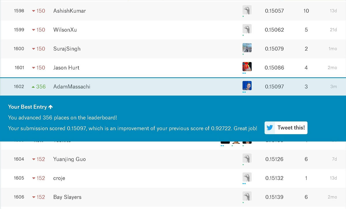
Our Submission!
我们的意见书!
We placed 1602 out of about 2400 competitors. Almost middle of the pack, not bad! Notice that our score here is .15097, which is better than the score we observed on the test data. That’s a good result, but will not always be the case.
我们在大约2400个竞争对手中排名1602。 几乎是背包的中间,还不错! 请注意,这里的分数是.15097 ,比我们在测试数据上观察到的分数要好。 这是一个很好的结果,但并非总是如此。
下一步 (Next steps)
You can extend this tutorial and improve your results by:
您可以通过以下方法扩展本教程并改善结果:
- Working with and transforming other features in the training set
- Experimenting with different modeling techniques, such as Random Forest Regressors or Gradient Boosting
- Using ensembling models
- 使用并转换训练集中的其他功能
- 实验不同的建模技术,例如随机森林回归器或梯度提升
- 使用集成模型
We created a set of categorical features called categoricals that were not all included in the final model. Go back and try to include these features. There are other methods that might help with categorical data, notably the pd.get_dummies() method. After working on these features, repeat the transformations for the test data and make another submission.
我们创建了一套名为类别特征categoricals了未全部包含在最终的模型。 返回并尝试包含这些功能。 还有其他可能有助于分类数据的方法,尤其是pd.get_dummies()方法。 使用完这些功能后,重复测试数据的转换并再次提交。
Working on models and participating in Kaggle competitions can be an iterative process – it’s important to experiment with new ideas, learn about the data, and test newer models and techniques.
制作模型和参加Kaggle比赛可能是一个反复的过程-尝试新想法,了解数据并测试更新的模型和技术非常重要。
翻译自: https://www.pybloggers.com/2017/05/getting-started-with-kaggle-house-prices-competition/
kaggle 入门


 1万+
1万+


 被折叠的 条评论
为什么被折叠?
被折叠的 条评论
为什么被折叠?
 到【灌水乐园】发言


