


 线性回归是一种统计模型,分析因变量与一组自变量间的线性关系。包括简单线性回归(SLR)和多元线性回归(MLR)。SLR使用单个特征预测响应,而MLR使用两个或更多特征。Python中可以使用scikit-learn库实现线性回归,同时模型假设数据中无多重共线性、自相关,并且响应与特征变量间存在线性关系。

线性回归算法
回归算法-线性回归 (Regression Algorithms - Linear Regression)
线性回归简介 (Introduction to Linear Regression)
Linear regression may be defined as the statistical model that analyzes the linear relationship between a dependent variable with given set of independent variables. Linear relationship between variables means that when the value of one or more independent variables will change (increase or decrease), the value of dependent variable will also change accordingly (increase or decrease).
线性回归可以定义为统计模型,用于分析因变量与给定的一组自变量之间的线性关系。 变量之间的线性关系意味着,当一个或多个自变量的值更改(增加或减少)时,因变量的值也将相应更改(增加或减少)。
Mathematically the relationship can be represented with the help of following equation −
数学上的关系可以借助以下方程式来表示-
Y = mX + b
Y = mX + b
Here, Y is the dependent variable we are trying to predict
在这里,Y是我们试图预测的因变量
X is the dependent variable we are using to make predictions.
X是我们用来进行预测的因变量。
m is the slop of the regression line which represents the effect X has on Y
m是回归线的斜率,代表X对Y的影响
b is a constant, known as the Y-intercept. If X = 0,Y would be equal to b.
b是一个常数,称为Y截距。 如果X = 0,则Y等于b。
Furthermore, the linear relationship can be positive or negative in nature as explained below −
此外,线性关系本质上可以是正或负,如下所述-
正线性关系 (Positive Linear Relationship)
A linear relationship will be called positive if both independent and dependent variable increases. It can be understood with the help of following graph −
如果自变量和因变量都增加,则线性关系称为正。 下图可以帮助理解-

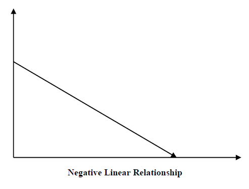
负线性关系 (Negative Linear relationship)
A linear relationship will be called positive if independent increases and dependent variable decreases. It can be understood with the help of following graph −
如果自增和因变量减小,则线性关系将称为正。 下图可以帮助理解-
线性回归的类型 (Types of Linear Regression)
Linear regression is of the following two types −
线性回归具有以下两种类型-
- Simple Linear Regression 简单线性回归
- Multiple Linear Regression 多元线性回归
简单线性回归(SLR) (Simple Linear Regression (SLR))
It is the most basic version of linear regression which predicts a response using a single feature. The assumption in SLR is that the two variables are linearly related.
它是线性回归的最基本版本,可使用单个功能预测响应。 SLR中的假设是两个变量线性相关。
Python实现 (Python implementation)
We can implement SLR in Python in two ways, one is to provide your own dataset and other is to use dataset from scikit-learn python library.
我们可以通过两种方式在Python中实现SLR,一种是提供自己的数据集,另一种是使用scikit-learn python库中的数据集。
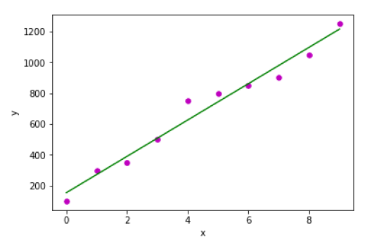
Example 1 − In the following Python implementation example, we are using our own dataset.
示例1-在下面的Python实现示例中,我们使用自己的数据集。
First, we will start with importing necessary packages as follows −
首先,我们将从导入必要的包开始,如下所示:
%matplotlib inline
import numpy as np
import matplotlib.pyplot as plt
Next, define a function which will calculate the important values for SLR −
接下来,定义一个函数,该函数将计算SLR的重要值-
def coef_estimation(x, y):
The following script line will give number of observations n −
以下脚本行将给出观察值n-
n = np.size(x)
The mean of x and y vector can be calculated as follows −
x和y向量的均值可以计算如下-
m_x, m_y = np.mean(x), np.mean(y)
We can find cross-deviation and deviation about x as follows −
我们可以找到关于x的交叉偏差和偏差,如下所示:
SS_xy = np.sum(y*x) - n*m_y*m_x
SS_xx = np.sum(x*x) - n*m_x*m_x
Next, regression coefficients i.e. b can be calculated as follows −
接下来,回归系数即b可以如下计算:
b_1 = SS_xy / SS_xx
b_0 = m_y - b_1*m_x
return(b_0, b_1)
Next, we need to define a function which will plot the regression line as well as will predict the response vector −
接下来,我们需要定义一个函数,该函数将绘制回归线以及预测响应向量-
def plot_regression_line(x, y, b):
The following script line will plot the actual points as scatter plot −
以下脚本行将实际点绘制为散点图-
plt.scatter(x, y, color = "m", marker = "o", s = 30)
The following script line will predict response vector −
以下脚本行将预测响应向量-
y_pred = b[0] + b[1]*x
The following script lines will plot the regression line and will put the labels on them −
以下脚本行将绘制回归线并在其上放置标签-
plt.plot(x, y_pred, color = "g")
plt.xlabel('x')
plt.ylabel('y')
plt.show()
At last, we need to define main() function for providing dataset and calling the function we defined above −
最后,我们需要定义main()函数以提供数据集并调用上面定义的函数-
def main():
   x = np.array([0, 1, 2, 3, 4, 5, 6, 7, 8, 9])
   y = np.array([100, 300, 350, 500, 750, 800, 850, 900, 1050, 1250])
   b = coef_estimation(x, y)
   print("Estimated coefficients:\nb_0 = {} \nb_1 = {}".format(b[0], b[1]))
   plot_regression_line(x, y, b)

if __name__ == "__main__":
main()
输出量 (Output)
Estimated coefficients:
b_0 = 154.5454545454545
b_1 = 117.87878787878788
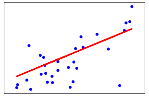
Example 2 − In the following Python implementation example, we are using diabetes dataset from scikit-learn.
示例2-在以下Python实现示例中,我们使用scikit-learn的糖尿病数据集。
First, we will start with importing necessary packages as follows −
首先,我们将从导入必要的包开始,如下所示:
%matplotlib inline
import matplotlib.pyplot as plt
import numpy as np
from sklearn import datasets, linear_model
from sklearn.metrics import mean_squared_error, r2_score
Next, we will load the diabetes dataset and create its object −
接下来,我们将加载糖尿病数据集并创建其对象-
diabetes = datasets.load_diabetes()
As we are implementing SLR, we will be using only one feature as follows −
在实现SLR时,我们将仅使用一种功能,如下所示-
X = diabetes.data[:, np.newaxis, 2]
Next, we need to split the data into training and testing sets as follows −
接下来,我们需要将数据分为以下训练集和测试集:
X_train = X[:-30]
X_test = X[-30:]
Next, we need to split the target into training and testing sets as follows −
接下来,我们需要将目标分为训练集和测试集,如下所示:
y_train = diabetes.target[:-30]
y_test = diabetes.target[-30:]
Now, to train the model we need to create linear regression object as follows −
现在,要训练模型,我们需要创建线性回归对象,如下所示:
regr = linear_model.LinearRegression()
Next, train the model using the training sets as follows −
接下来,使用以下训练集训练模型:
regr.fit(X_train, y_train)
Next, make predictions using the testing set as follows −
接下来,使用测试集进行预测,如下所示:
y_pred = regr.predict(X_test)
Next, we will be printing some coefficient like MSE, Variance score etc. as follows −
接下来,我们将打印一些系数,例如MSE,方差得分等,如下所示-
print('Coefficients: \n', regr.coef_)
print("Mean squared error: %.2f" % mean_squared_error(y_test, y_pred))
print('Variance score: %.2f' % r2_score(y_test, y_pred))
Now, plot the outputs as follows −
现在,绘制输出,如下所示:
plt.scatter(X_test, y_test, color='blue')
plt.plot(X_test, y_pred, color='red', linewidth=3)
plt.xticks(())
plt.yticks(())
plt.show()
输出量 (Output)
Coefficients:
   [941.43097333]
Mean squared error: 3035.06
Variance score: 0.41
多元线性回归(MLR) (Multiple Linear Regression (MLR))
It is the extension of simple linear regression that predicts a response using two or more features. Mathematically we can explain it as follows −
简单线性回归的扩展是使用两个或多个功能预测响应的方法。 数学上,我们可以解释如下-
Consider a dataset having n observations, p features i.e. independent variables and y as one response i.e. dependent variable the regression line for p features can be calculated as follows −
$$h(x_{i})=b_{0}+b_{1}x_{i1}+b_{2}x_{i2}+...+b_{p}x_{ip}$$考虑具有n个观测值,p个特征(即自变量)和y作为一个响应(即因变量)的数据集,p个特征的回归线可以如下计算:
$$ h(x_ {i})= b_ {0} + b_ {1} x_ {i1} + b_ {2} x_ {i2} + ... + b_ {p} x_ {ip} $$Here, h(xi) is the predicted response value and b0,b1,b2…,bp are the regression coefficients.
在此,h(x i )是预测响应值,b 0 ,b 1 ,b 2 …,b p是回归系数。
Multiple Linear Regression models always includes the errors in the data known as residual error which changes the calculation as follows −
$$h(x_{i})=b_{0}+b_{1}x_{i1}+b_{2}x_{i2}+...+b_{p}x_{ip}+e_{i}$$多个线性回归模型始终将数据中的误差称为残留误差,该误差会按以下方式更改计算:
$$ h(x_ {i})= b_ {0} + b_ {1} x_ {i1} + b_ {2} x_ {i2} + ... + b_ {p} x_ {ip} + e_ {i} $$We can also write the above equation as follows −
$$y_{i}=h(x_{i})+e_{i}\:or\:e_{i}= y_{i} - h(x_{i})$$我们还可以将上面的等式写成如下-
$$ y_ {i} = h(x_ {i})+ e_ {i} \:or \:e_ {i} = y_ {i}-h(x_ {i})$$Python实现 (Python Implementation)
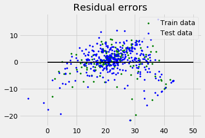
in this example, we will be using Boston housing dataset from scikit learn −
在此示例中,我们将使用来自scikit learning的Boston住房数据集-
First, we will start with importing necessary packages as follows −
首先,我们将从导入必要的包开始,如下所示:
%matplotlib inline
import matplotlib.pyplot as plt
import numpy as np
from sklearn import datasets, linear_model, metrics
Next, load the dataset as follows −
接下来,按如下方式加载数据集:
boston = datasets.load_boston(return_X_y=False)
The following script lines will define feature matrix, X and response vector, Y −
以下脚本行将定义特征矩阵X和响应向量Y-
X = boston.data
y = boston.target
Next, split the dataset into training and testing sets as follows −
接下来,将数据集分为训练集和测试集,如下所示:
from sklearn.model_selection import train_test_split
X_train, X_test, y_train, y_test = train_test_split(X, y, test_size=0.7, random_state=1)
例 (Example)
Now, create linear regression object and train the model as follows −
现在,创建线性回归对象并按如下所示训练模型-
reg = linear_model.LinearRegression()
reg.fit(X_train, y_train)
print('Coefficients: \n', reg.coef_)
print('Variance score: {}'.format(reg.score(X_test, y_test)))
plt.style.use('fivethirtyeight')
plt.scatter(reg.predict(X_train), reg.predict(X_train) - y_train,
   color = "green", s = 10, label = 'Train data')
plt.scatter(reg.predict(X_test), reg.predict(X_test) - y_test,
   color = "blue", s = 10, label = 'Test data')
plt.hlines(y = 0, xmin = 0, xmax = 50, linewidth = 2)
plt.legend(loc = 'upper right')
plt.title("Residual errors")
plt.show()
输出量 (Output)
Coefficients:
[
   -1.16358797e-01  6.44549228e-02  1.65416147e-01  1.45101654e+00
   -1.77862563e+01  2.80392779e+00  4.61905315e-02 -1.13518865e+00
    3.31725870e-01 -1.01196059e-02 -9.94812678e-01  9.18522056e-03
   -7.92395217e-01
]
Variance score: 0.709454060230326
假设条件 (Assumptions)
The following are some assumptions about dataset that is made by Linear Regression model −
以下是关于由线性回归模型建立的数据集的一些假设-
Multi-collinearity − Linear regression model assumes that there is very little or no multi-collinearity in the data. Basically, multi-collinearity occurs when the independent variables or features have dependency in them.
多重共线性 -线性回归模型假设数据中很少或没有多重共线性。 基本上,当自变量或要素具有相关性时,就会发生多重共线性。
Auto-correlation − Another assumption Linear regression model assumes is that there is very little or no auto-correlation in the data. Basically, auto-correlation occurs when there is dependency between residual errors.
自相关 -另一个假设是线性回归模型所假设的是,数据中几乎没有自相关。 基本上,当残差之间存在依赖性时,就会发生自相关。
Relationship between variables − Linear regression model assumes that the relationship between response and feature variables must be linear.
变量之间的关系 -线性回归模型假定响应变量和特征变量之间的关系必须是线性的。
线性回归算法


 1795
1795

 被折叠的 条评论
为什么被折叠?
被折叠的 条评论
为什么被折叠?
 到【灌水乐园】发言


