论文 A Linear Time Algorithm for Placing phi-Nodes：阅读笔记

介绍

这个论文提出了一种简单高效率的插入$\varphi$-node的方法，也指出了传统插入$\varphi$-node算法的一些弊端。
注：这个论文还有一些前置论文，我懒得看了

想要解决的问题

论文想要解决的是在计算dominance frontier时候潜在的$O(N^2)$的复杂度。论文指出计算$\varphi$-node插入位置可以在线性时间内完成，核心就在于处理dominator tree的顺序，同时这种方式还可以on-the-fly的方式计算dominance frontier。

该论文使用了一种$DJ-graph$的结构来作为整个算法的基础。DJ-Graph的本质上是在dominator tree上添加了J-edge（join-edge），

The tree skeleton is augmented with J-edges (join edges) that correspond to all edges of the CFG whose source does not strictly dominate its destination. - Static Single Assignment Book

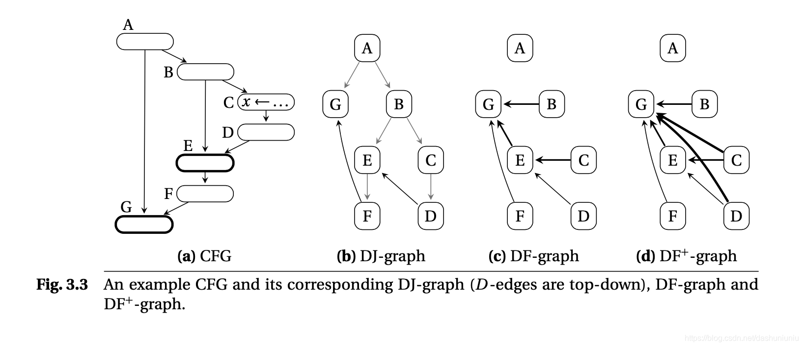
注：上图源于Static Single Assignment Book

传统placing $\varphi$-node算法回顾

在构造SSA介绍的插入$\varphi$-node的算法比较粗糙，还没有考虑到live信息，效率也比较低。

注：上图来自于Data Flow Analysis Theory and Pratice

这个算法有两个特点，一是预先计算好所有的dominance frontier信息，二是迭代的方式插入$\varphi$-node的效率比较低。

背景知识

有两点背景知识以前没有接触过，一个是dominance frontier的拓展，从一个节点的$DF(x)$ 拓展到一个节点集合 $DF(S)$。

$$DF(S)=\bigcup _{x\in S}DF(x)$$

另一个是iterated dominance frontier $IDF(S)$或者（$D{F}^{+}(S$）（这也是我为什么看llvm的代码IDFCalculatorBase看不懂的原因 😃）,$IDS(S)$是通过迭代计算$DF(S)$得到的，其实也就是$DF$的传递闭包。

$$\begin{gathered} ID{F}_1(S)=DF(S) \\ ID{F}_{i+1}=DF(S\cup ID{F}_i(S)) \end{gathered}$$

其实在传统的$\varphi$-node插入算法中，迭代就是为了计算这个$IDF(S)$。

另外，对于$J-edge(a,b)$，所有$a$ DT上的ancestors（包括$a$）也不会strictly dominate $b$，也就是$b$也在这些ancestor的DF集合中。例如Fig3.3中，($F$, $G$)是一个$J-edge$，所有{($F$, $G$), ($E$, $G$), ($B$, $G$)}也是$DF-edge$。

那么$J-edge$和$DF$的关系是$DF$可以有简单的$J-edge$推出来。

核心实现

首先$DJ-graph$有几个需要在着重强调的特性，

线性时间构造DJ-graph

注：上图来源于论文

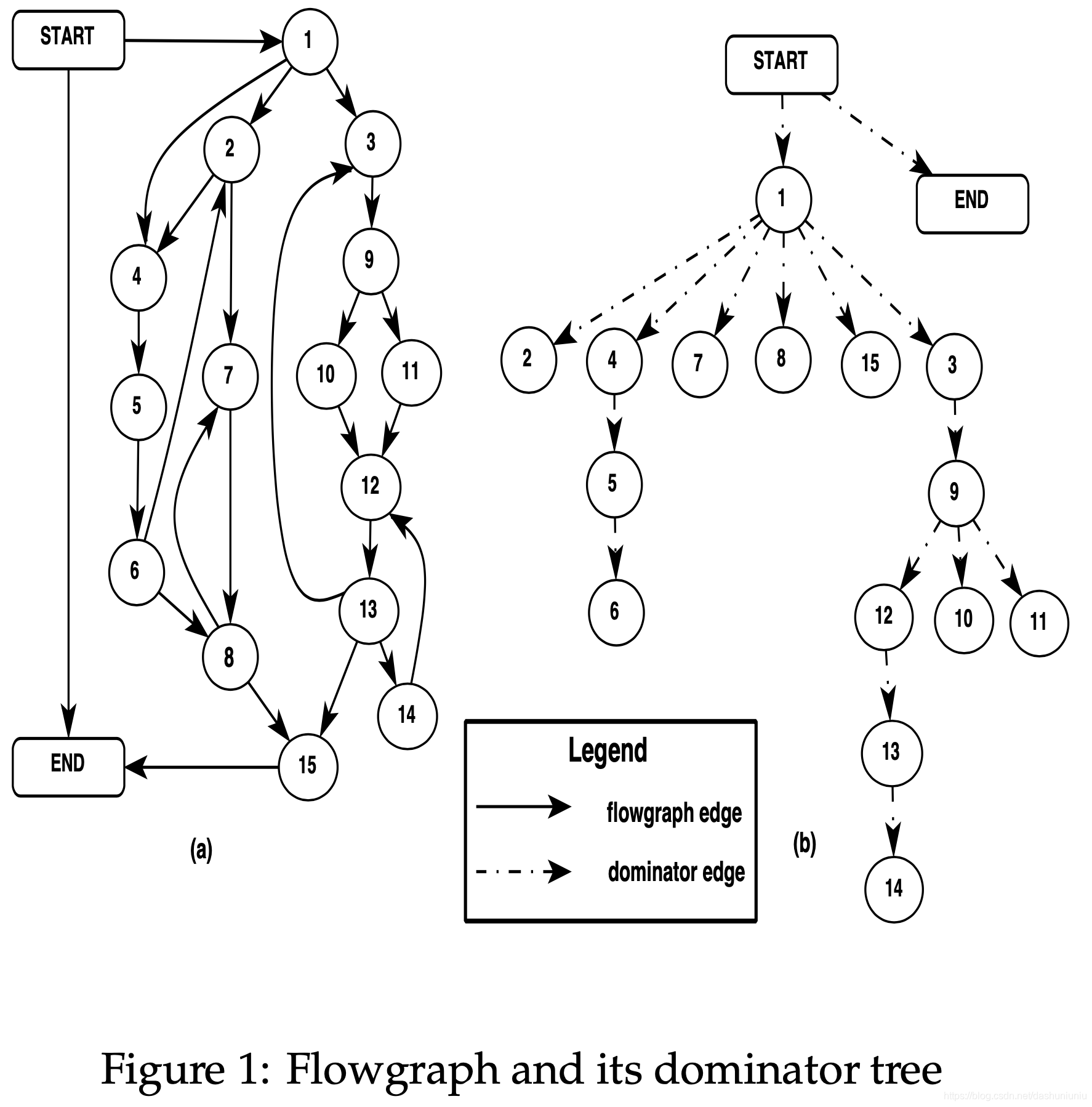
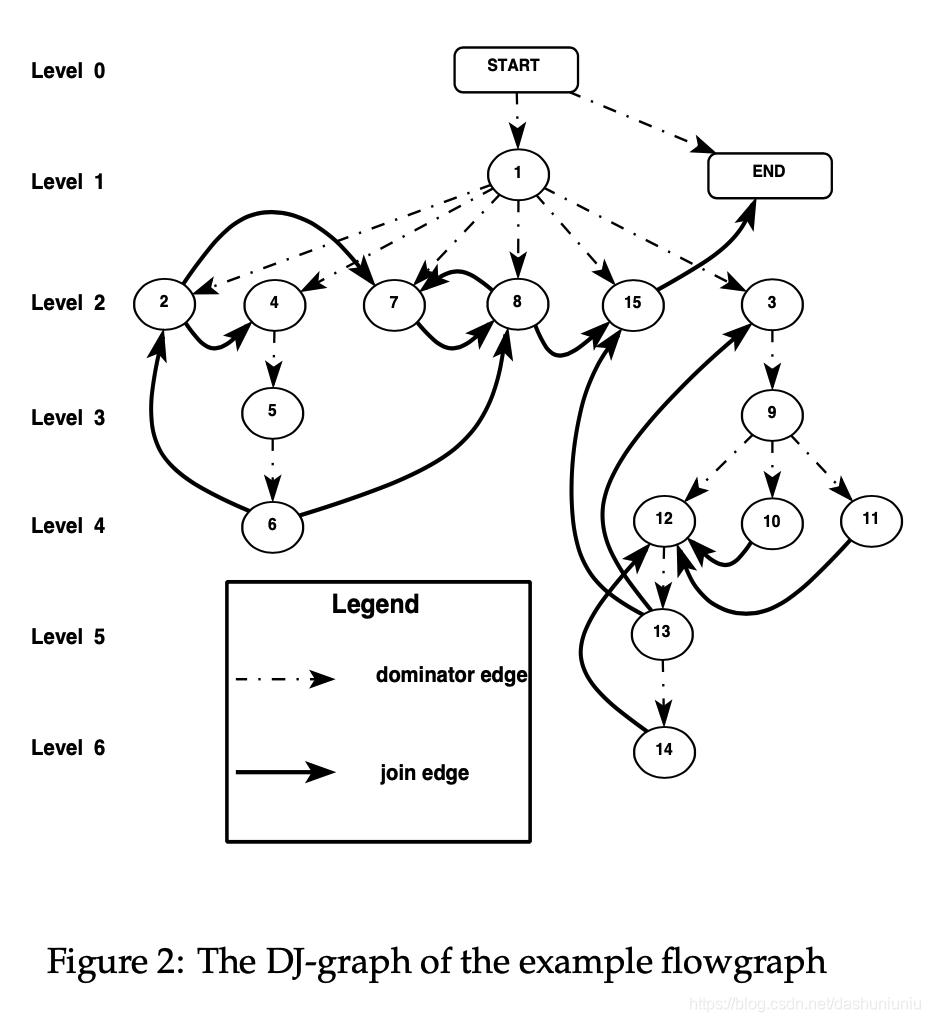
首先$DJ-graph$以dominator tree作为骨架，第一点就是在其上添加join edges，例如我们要为Figure 2中的节点2附着join edge，首先在flowgraph中找到destination为节点2的边，例如$1\to 2$和$2\to 6$，但是$1$支配$2$，所以我们在dominator tree加上$6\to 2$。只要我们考察完flowgraph所有的边，再结合dominator tree就可以在构造出$DJ-graph$。

$DJ-graph$有以下三个属性：

• 前面我们已经探讨了$J$ edge 和dominance frontier的关系，例如对于$J-edge(a,b)$，$b$在所有$a$及其ancestor的$DF$集合中。
• 对于$y\in DF(x)$（同样$y\in IDF(x)$），$y$在dominator tree中的level永远小于等于$x$。这是整篇论文的关键，换句话说，如果我们要找$x$的dominance fontier，只找level值小于等于$x$的节点就够了。
• $y\in DF(x)$，当且仅当存在$z\in SubTree(x)$，并且存在一条$J-edge$ $z\to y$同时$y$的level值小于等于$x$的level值。

computing dominance frontier

论文推出了一条引理，

Lemma 1 : A node $z\in DF(x)$ iff there exists a $y\in SubTree(x)$ with $y\to z$ as a $J-edge$ and $z.level\le x.level$

通过上面的引理论文给出了一个计算dominance frontier的算法，

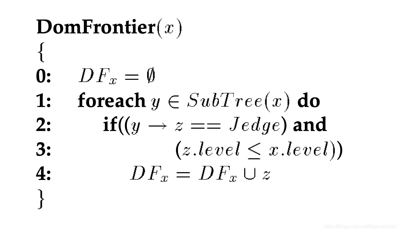
例如我们要计算Figure 2中节点$3$的dominance frontier，首先$SubTree(3)=3,9,10,11,12,13,14$，$J-edge$有$10\to 12,11\to 12,13\to 3,13\to 15,14\to 12$。而其中节点$3$，$15$满足上面的引理，所以$DF(3)=3,15$。

该篇论文算法的另一个核心就是顺序，例如我们要计算$DF(9,12)$，因为$12\in SubTree(9)$，所以我们在计算dominance frontier时，节点$12$的$SubTree$被处理了两遍，所以在计算dominance frontier时按照dominator tree的level从下到上处理。

如下图所示，在处理$DF(w)$之前，$DF(x)$已经计算出来了。

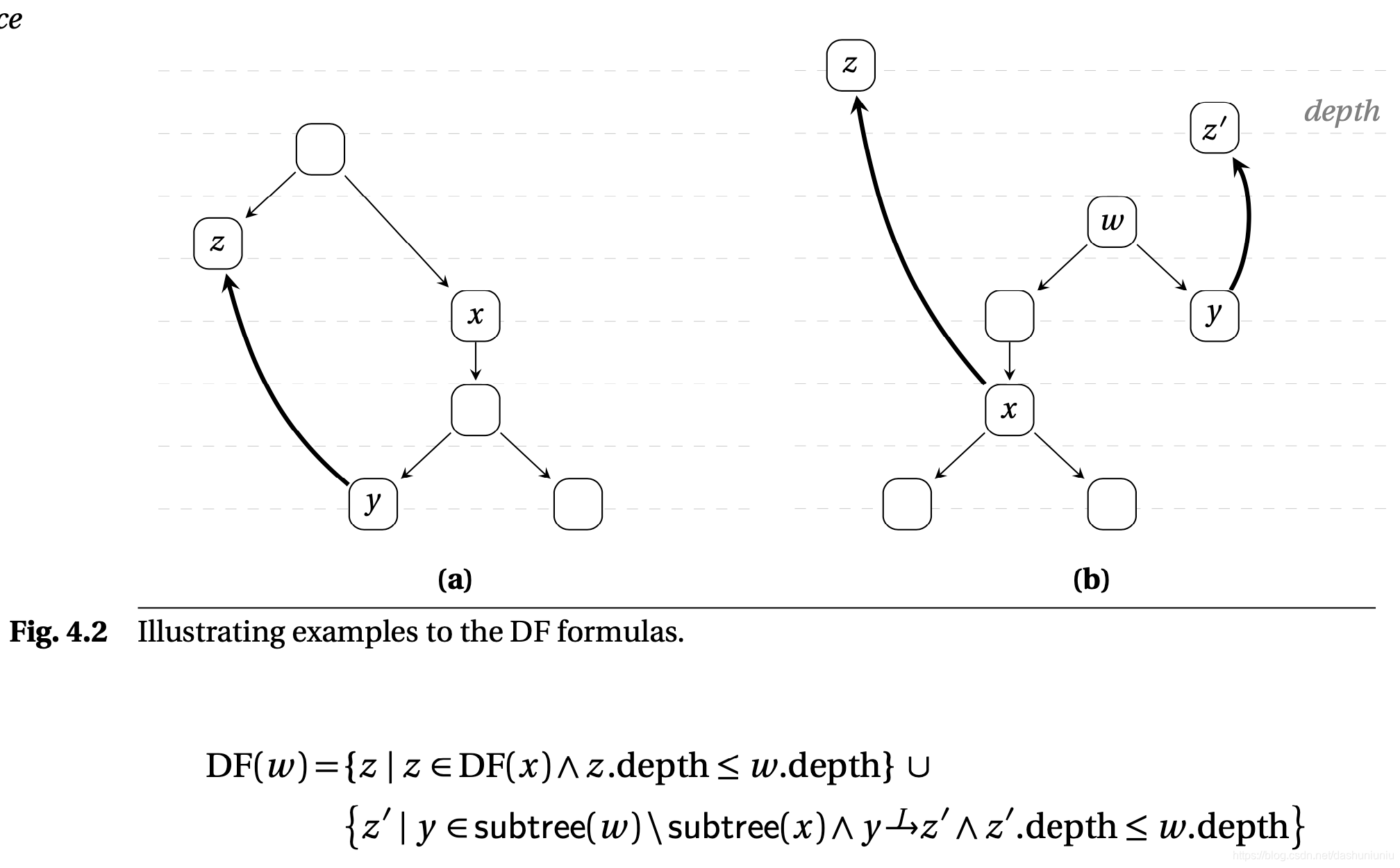
注：上图来自与Static Single Assignment Book

插入$\varphi$-node

在我们得到$DJ-graph$之后，就可以计算$\varphi$-node插入的位置。这里的算法使用《Static Single Assignment Book》的描述。

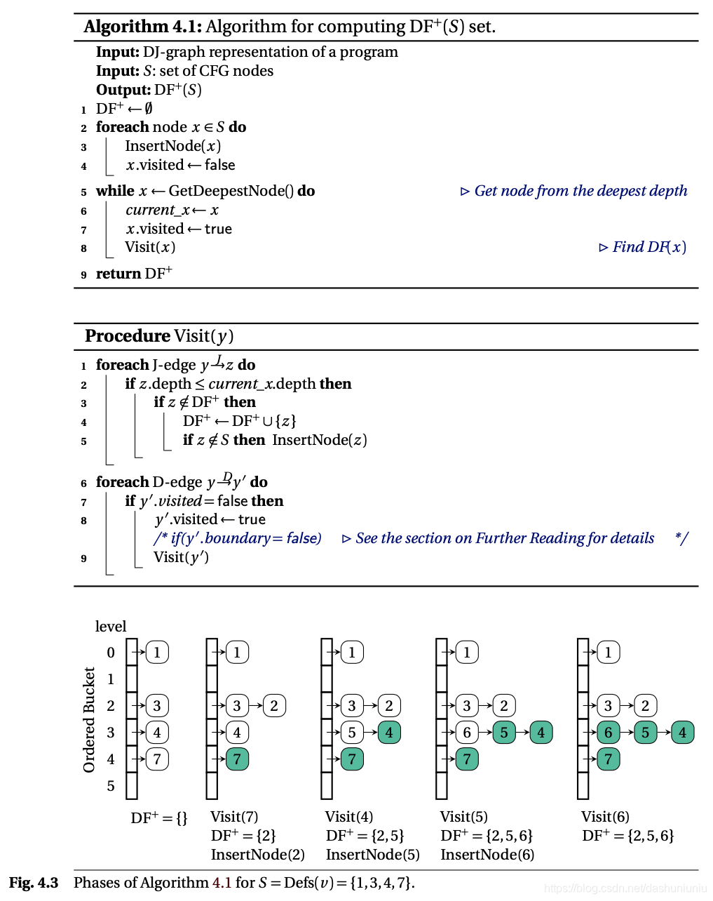
例如对$v$进行定义的节点有$1$，$3$，$4$，$7$。首先算法使用一个$OrderedBucket$来组织这些节点，然后按照depth从大到小处理以这些节点为起始点的$J$-edge，如果这个edge满足引理Lemma 1，则把$J$-edge的终止节点加入$DF(1,3,4,7)$中。

这篇论文的算法针对《构造SSA》的改进有以下几点：

• 把计算dominance frontier的粒度从单个节点扩展到一个节点集合。例如对于变量$x$的$def$通常也是一个节点集合。
• 不需要预先计算dominance frontier，可以on-the-fly地计算dominance frontier
• 通过$J$-edge，以bottom up的方式地进行处理，保证每个节点每条边只处理一遍没提升了效率

效果及使用情况

通过论文作者的描述，该算法实现了5倍的提升。llvm最开始的时候使用的是Cytron的算法，后来就使用本论文中的算法，见GenericIteratedDominanceFrontier.h。

//===- IteratedDominanceFrontier.h - Calculate IDF ------------*- C++ -*-===//
//
// Compute iterated dominance frontiers using a linear time algorithm.
//
// The algorithm used here is based on:
//
//  Sreedhar and Gao. A linear time algorithm for placing phi-nodes.
//  In Proceedings of the 22nd ACM SIGPLAN-SIGACT Symposium on Principles of
//  Programming Languages
//  POPL '95. ACM, New York, NY, 62-73.
//
// It has been modified to not explicitly use the DJ graph data structure and
// to directly compute pruned SSA using per-veriable liveness information.
//
//===--------------------------------------------------------------------===//