吴恩达团队 Tensorflow课程学习笔记 1

kaggle上的猫狗识别分类比赛

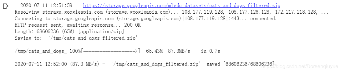
下载图像集

简介

图像集来自于kaggle的猫狗大赛的数据集，可以直接下载，为了方便学习，只用了其中的一部分。它们存储为zip文件，其中包含3000张图片，我们将其中的2000张用于训练，1000张用于测试

!wget --no-check-certificate \
  https://storage.googleapis.com/mledu-datasets/cats_and_dogs_filtered.zip \
  -O /tmp/cats_and_dogs_filtered.zip

下载结果

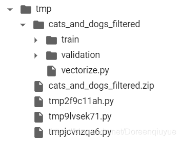
文件解压

import os
import zipfile

local_zip = '/tmp/cats_and_dogs_filtered.zip'

zip_ref = zipfile.ZipFile(local_zip, 'r')

zip_ref.extractall('/tmp')
zip_ref.close()

设置目录

其中子目录将被重新创建，因为它们存储在压缩文件里
设置目录作为变量，方便后续将生成器指向它们

base_dir = '/tmp/cats_and_dogs_filtered'

train_dir = os.path.join(base_dir, 'train')
validation_dir = os.path.join(base_dir, 'validation')

# Directory with our training cat/dog pictures
train_cats_dir = os.path.join(train_dir, 'cats')
train_dogs_dir = os.path.join(train_dir, 'dogs')

# Directory with our validation cat/dog pictures
validation_cats_dir = os.path.join(validation_dir, 'cats')
validation_dogs_dir = os.path.join(validation_dir, 'dogs')

目录分布

查看图片路径

将这些变量传给os.listdir，从这些目录中提取文件，并将它们加载到python列表中

train_cat_fnames = os.listdir( train_cats_dir )
train_dog_fnames = os.listdir( train_dogs_dir )

print(train_cat_fnames[:10])
print(train_dog_fnames[:10])

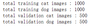
查看图片数量

print('total training cat images :', len(os.listdir(      train_cats_dir ) ))
print('total training dog images :', len(os.listdir(      train_dogs_dir ) ))

print('total validation cat images :', len(os.listdir( validation_cats_dir ) ))
print('total validation dog images :', len(os.listdir( validation_dogs_dir ) ))

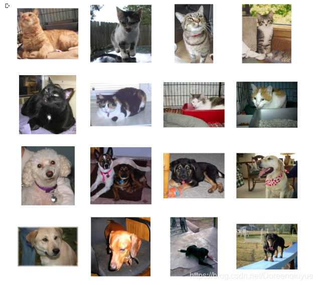
结果展示

图像可视化

随机挑选一些猫狗，并绘制在网格中

%matplotlib inline

import matplotlib.image as mpimg
import matplotlib.pyplot as plt

# Parameters for our graph; we'll output images in a 4x4 configuration
nrows = 4
ncols = 4

pic_index = 0 # Index for iterating over images

fig = plt.gcf()
fig.set_size_inches(ncols*4, nrows*4)

pic_index+=8

next_cat_pix = [os.path.join(train_cats_dir, fname) 
                for fname in train_cat_fnames[ pic_index-8:pic_index] 
               ]

next_dog_pix = [os.path.join(train_dogs_dir, fname) 
                for fname in train_dog_fnames[ pic_index-8:pic_index]
               ]

for i, img_path in enumerate(next_cat_pix+next_dog_pix):
  # Set up subplot; subplot indices start at 1
  sp = plt.subplot(nrows, ncols, i + 1)
  sp.axis('Off') # Don't show axes (or gridlines)

  img = mpimg.imread(img_path)
  plt.imshow(img)

plt.show()

搭建神经网络

导入Tensorflow

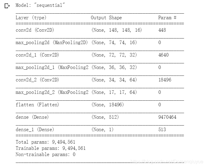
定义模型

打印摘要

import tensorflow as tf
model = tf.keras.models.Sequential([
    # Note the input shape is the desired size of the image 150x150 with 3 bytes color
    tf.keras.layers.Conv2D(16, (3,3), activation='relu', input_shape=(150, 150, 3)),
    tf.keras.layers.MaxPooling2D(2,2),
    tf.keras.layers.Conv2D(32, (3,3), activation='relu'),
    tf.keras.layers.MaxPooling2D(2,2), 
    tf.keras.layers.Conv2D(64, (3,3), activation='relu'), 
    tf.keras.layers.MaxPooling2D(2,2),
    # Flatten the results to feed into a DNN
    tf.keras.layers.Flatten(), 
    # 512 neuron hidden layer
    tf.keras.layers.Dense(512, activation='relu'), 
    # Only 1 output neuron. It will contain a value from 0-1 where 0 for 1 class ('cats') and 1 for the other ('dogs')
    tf.keras.layers.Dense(1, activation='sigmoid')  
])

model.summary()

编译模型

from tensorflow.keras.optimizers import RMSprop

model.compile(optimizer=RMSprop(lr=0.001),
              loss='binary_crossentropy',
              metrics = ['acc'])

生成器

设置两个生成器，指向对应目录

from tensorflow.keras.preprocessing.image import ImageDataGenerator

# All images will be rescaled by 1./255.
train_datagen = ImageDataGenerator( rescale = 1.0/255. )
test_datagen  = ImageDataGenerator( rescale = 1.0/255. )

# --------------------
# Flow training images in batches of 20 using train_datagen generator
# --------------------
train_generator = train_datagen.flow_from_directory(train_dir,
                                                    batch_size=20,
                                                    class_mode='binary',
                                                    target_size=(150, 150))     
# --------------------
# Flow validation images in batches of 20 using test_datagen generator
# --------------------
validation_generator =  test_datagen.flow_from_directory(validation_dir,
                                                         batch_size=20,
                                                         class_mode  = 'binary',
                                                         target_size = (150, 150))

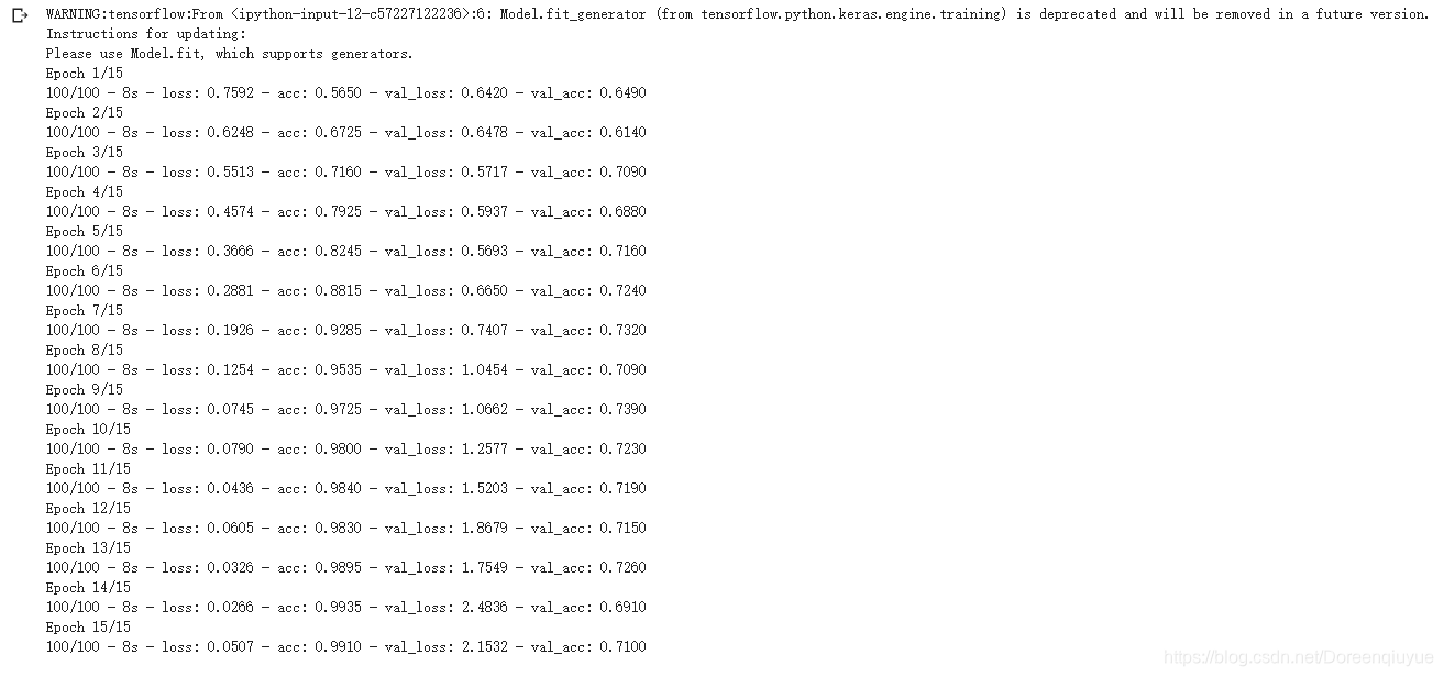
模型训练

数据源是生成器，所以训练用的是model.fit_generator

history = model.fit_generator(train_generator,
                              validation_data=validation_generator,
                              steps_per_epoch=100,
                              epochs=15,
                              validation_steps=50,
                              verbose=2)

模型测试

import numpy as np

from google.colab import files
from keras.preprocessing import image

uploaded=files.upload()

for fn in uploaded.keys():
 
  # predicting images
  path='/content/' + fn
  img=image.load_img(path, target_size=(150, 150))
  
  x=image.img_to_array(img)
  x=np.expand_dims(x, axis=0)
  images = np.vstack([x])
  
  classes = model.predict(images, batch_size=10)
  
  print(classes[0])
  
  if classes[0]>0:
    print(fn + " is a dog")
    
  else:
    print(fn + " is a cat")

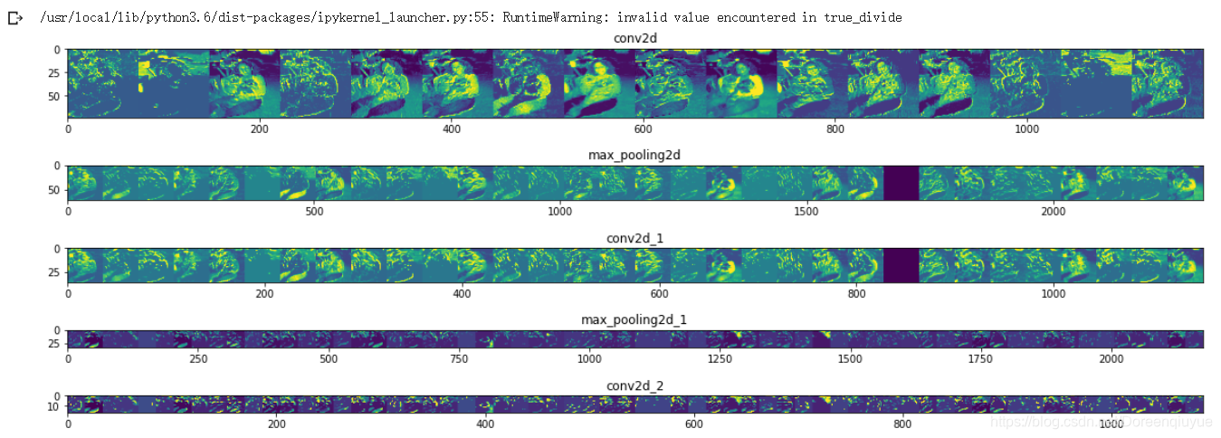
可视化卷积中间结果图

import numpy as np
import random
from   tensorflow.keras.preprocessing.image import img_to_array, load_img

# Let's define a new Model that will take an image as input, and will output
# intermediate representations for all layers in the previous model after
# the first.
successive_outputs = [layer.output for layer in model.layers[1:]]

#visualization_model = Model(img_input, successive_outputs)
visualization_model = tf.keras.models.Model(inputs = model.input, outputs = successive_outputs)

# Let's prepare a random input image of a cat or dog from the training set.
cat_img_files = [os.path.join(train_cats_dir, f) for f in train_cat_fnames]
dog_img_files = [os.path.join(train_dogs_dir, f) for f in train_dog_fnames]

img_path = random.choice(cat_img_files + dog_img_files)
img = load_img(img_path, target_size=(150, 150))  # this is a PIL image

x   = img_to_array(img)                           # Numpy array with shape (150, 150, 3)
x   = x.reshape((1,) + x.shape)                   # Numpy array with shape (1, 150, 150, 3)

# Rescale by 1/255
x /= 255.0

# Let's run our image through our network, thus obtaining all
# intermediate representations for this image.
successive_feature_maps = visualization_model.predict(x)

# These are the names of the layers, so can have them as part of our plot
layer_names = [layer.name for layer in model.layers]

# -----------------------------------------------------------------------
# Now let's display our representations
# -----------------------------------------------------------------------
for layer_name, feature_map in zip(layer_names, successive_feature_maps):
  
  if len(feature_map.shape) == 4:
    
    #-------------------------------------------
    # Just do this for the conv / maxpool layers, not the fully-connected layers
    #-------------------------------------------
    n_features = feature_map.shape[-1]  # number of features in the feature map
    size       = feature_map.shape[ 1]  # feature map shape (1, size, size, n_features)
    
    # We will tile our images in this matrix
    display_grid = np.zeros((size, size * n_features))
    
    #-------------------------------------------------
    # Postprocess the feature to be visually palatable
    #-------------------------------------------------
    for i in range(n_features):
      x  = feature_map[0, :, :, i]
      x -= x.mean()
      x /= x.std ()
      x *=  64
      x += 128
      x  = np.clip(x, 0, 255).astype('uint8')
      display_grid[:, i * size : (i + 1) * size] = x # Tile each filter into a horizontal grid

    #-----------------
    # Display the grid
    #-----------------

    scale = 20. / n_features
    plt.figure( figsize=(scale * n_features, scale) )
    plt.title ( layer_name )
    plt.grid  ( False )
    plt.imshow( display_grid, aspect='auto', cmap='viridis' ) 

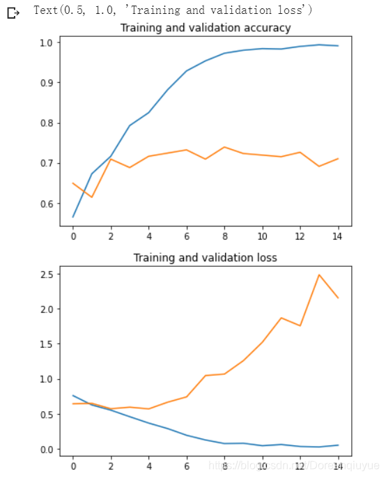
评估模型的精确度和损失

acc      = history.history[     'acc' ]
val_acc  = history.history[ 'val_acc' ]
loss     = history.history[    'loss' ]
val_loss = history.history['val_loss' ]

epochs   = range(len(acc)) # Get number of epochs

#------------------------------------------------
# Plot training and validation accuracy per epoch
#------------------------------------------------
plt.plot  ( epochs,     acc )
plt.plot  ( epochs, val_acc )
plt.title ('Training and validation accuracy')
plt.figure()

#------------------------------------------------
# Plot training and validation loss per epoch
#------------------------------------------------
plt.plot  ( epochs,     loss )
plt.plot  ( epochs, val_loss )
plt.title ('Training and validation loss'   )