Neural Networks: Learning: Putting it together_neural network learning algorithms-CSDN博客

本文链接：https://blog.csdn.net/edward_wang1/article/details/106505406

本文概述了吴恩达教授的神经网络学习算法，详细解释了如何选择网络架构，包括输入、隐藏和输出层单元数量的确定。文章还介绍了训练神经网络的六个步骤：初始化权重、实现前向传播、计算成本函数、实现反向传播、梯度检查和优化算法应用。

摘要生成于 C知道，由 DeepSeek-R1 满血版支持，前往体验 >

摘要: 本文是吴恩达 (Andrew Ng)老师《机器学习》课程，第十章《神经网络参数的反向传播算法》中第78课时《组合到一起》的视频原文字幕。为本人在视频学习过程中记录下来并加以修正，使其更加简洁，方便阅读，以便日后查阅使用。现分享给大家。如有错误，欢迎大家批评指正，在此表示诚挚地感谢！同时希望对大家的学习能有所帮助.
————————————————
So, it's taken us a lot of videos to get through the neural network learning algorithm. In this video, what I'd like to do is try to put all the pieces together, to give an overall summary or a bigger picture view, of how all the pieces fit together and of the overall process of how to implement a neural network learning algorithm.

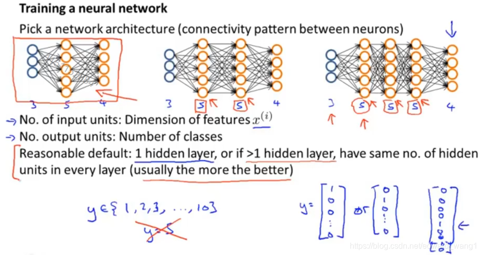
When training a neural network, the first thing you need to do is pick some network architecture and by architecture I just mean connectivity pattern between the neurons. So we might choose between say, a neural network with three input units and five hidden units and four output units versus one of 3, 5 hidden, 5 hidden, 4 output and here are 3, 5, 5, 5 units in each of three hidden units and 4 output units. And so these choices of how many hidden units in each layer and how many hidden layers, those are architecture choices. So how do you make these choices? Well first, the number of input units well that's pretty well defined. And once you decided on the fix set of features $x^{(i)}$ , the number of input units will just be the dimension of your features $x^{(i)}$ . It would be determined by that. And if you are doing multi-class classifications the number of output units will be determined by the number of classes in your classification problem. And just a reminder, if you have a multiclass classification where y takes on say values between 1 and 10 ( $y\in {1,2,3...,10}}$ ), so that you have 10 possible classes. Then remember to rewrite your output y as these vectors. So instead of class one, you re-code it as a vector like that $y=\begin{bmatrix} 1\\ 0\\ 0\\ .\\ .\\ .\\ 0\\ \end{bmatrix}$ , or for the second class you re-code it as a vector like that $y=\begin{bmatrix} 0\\ 1\\ 0\\ .\\ .\\ .\\ 0\\ \end{bmatrix}$ . So if one of these examples takes on the fifth class, you know, y equals 5, then what you're showing to your neural network is not a value of y equals 5, instead here at the output layer which would have 10 output units, you will instead feed to the vector with one in the fifth position and a bunch of zeros down here $y=\begin{bmatrix} 0\\ 0\\ 0\\ 0\\ 1\\ ...\\ 0\\ \end{bmatrix}$ . So the choice of number of input units and number of output units is maybe somewhat reasonably straightforward. And as for the number of hidden units and the number of hidden layers, a reasonable default is to use a single hidden layer, so this type of neural network shown on the left with just one hidden layer is probably the most common. Or if you use more than one hidden layer, again a reasonable default will be to have the same number of hidden units in every single layer. So here we have two hidden layers and each of these hidden layers has the same number five of hidden units and here we have three hidden layers and each of them has the same number, that is five hidden units. But rather than doing this, this sort of network architecture on the left would be a perfectly reasonable default. And as for the number of hidden units, usually, the more hidden units the better. It's just that if you have a lot of hidden units, it can become more computationally expensive, but very often, having more hidden units is good thing. And usually the number of hidden units in each layer will be maybe comparable to the dimension of x, comparable to the number of features, or it could be any where from same number of hidden units of input features to maybe twice of that three or four times of that. So having the number of hidden units, that is comparable or several times, or somewhat bigger than the number of input features, is often a useful thing to do. So, hopefully this gives you one reasonable set of default choices for network architecture, and if you follow these guidelines, you will probably get something that works well, but in a late set of videos where I will talk specifically about advice for how to apply algorithms, I will actually say a lot about how to choose a neural network architecture. Actually I have quite a lot more to say later about how to make good choices for the number of hidden units, the number of hidden layers and so on.

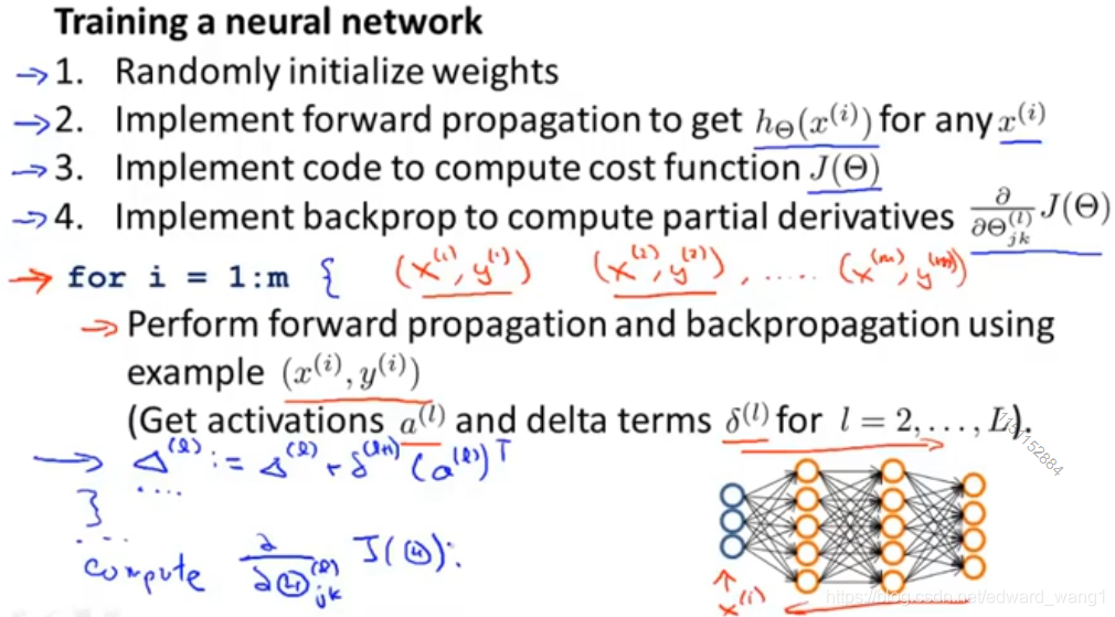
Next, here's what we need to implement in order to train a neural network, there are actually six steps and that I have four on this side and two more steps on the next slide. First step is setup the neural network and to randomly initialize the values of the weights. And we usually initialize the weights to small values near zero. Then we implement forward propagation so that we can input any input $x^{(i)}$ into neural network and compute $h_{\theta }(x^{(i)})$ which is the output vector of the y values. We then also implement code to compute this cost function $J(\Theta )$ . And next we implement backprop or the back propagation algorithm to compute these partial derivative terms $\frac{\partial }{\theta ^{(l)}_{jk}}J(\Theta )$ . Concretely, to implement back prop, usually we will do that with a for loop over the training examples. Some of you may have heard of advanced, and frankly very advanced vectorization methods where you don't have a for loop over the m training examples, but the first time you're implementing back prop there should almost certainly be a for loop in your code, where you're iterating over the examples, you know, $(x^{(1)},y^{(1)})$ , then so you do forward prop and back prop on the first example, and then in the second iteration of the for loop, you do forward propagation and back propagation on the second example $(x^{(2)},y^{(2)})$ , and so on, until you get through the final example $(x^{(m)},y^{(m)})$ . So there should be a for loop in your implementation of back prop at least first time implementing it. And then there are frankly somewhat complicated ways to do this without a for loop, but I definitely do not recommend trying to do that much more complicated version the first time you try to implement back prop. So concretely, we have a for loop over my m training examples and inside the for loop we're going to perform forward prop and back prop using just this one example ( $(x^{(i)},y^{(i)})$ ). And what that means is that we're going to take $x^{(i)}$ , and feed that to my input layer, perform forward prop, perform back prop, and that will give me all of these activations and all of these delta terms for all of the layers of all my units in the neural network. Then still inside this loop, let me draw some curly braces, just to show the scope of the loop, this is an Octave code of course, but just more like C++ or Java code, and a for loop encompasses all this. We're going to compute those delta terms, here's the formula that we gave earlier ( $\Delta ^{(l)}=\Delta ^{(l)}+\delta ^{l+1}(a^{(l)})^{T}$ ). And then finally, outside the for loop, having computed these delta terms, these accumulation terms, we would then have some other code and that will allow us to compute these partial derivative terms. And these partial derivatives have to take into account the regularization term $\lambda$ as well. Those formulas were given in the earlier video. So, having done that, you now hopefully have code to compute these partial derivative terms.

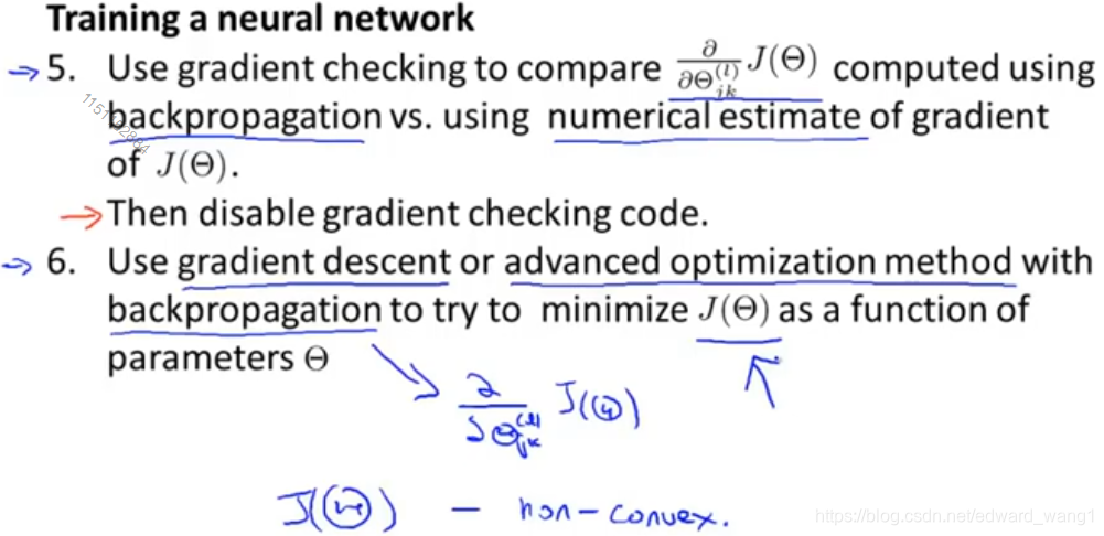
Next is step 5, what I do is then use gradient checking to compare these partial derivative terms that were computed. So, I've compared the version computed using back propagation versus the partial derivatives computed using the numerical estimates of the derivatives. So, I do gradient checking to make sure that both of these give you very similar values. Having done gradient checking just now reassures us that our implementation of back propagation is correct, and then is very important that we disable gradient checking, because gradient checking code is computationally very slow. And finally, we then use an optimization algorithm such as gradient descent, or one of the advanced optimization methods such as LBFGS, conjugate gradient as embodied into fminunc or other optimization methods. We use these together with back propagation, so back propagation is the thing that computes these partial derivatives for us. And so, we know how to compute the cost function, we know how to compute the partial derivatives using back propagation, so we can use one of the optimization methods to try to minimize $J(\Theta )$ . And by the way, for neural networks, this cost function $J(\Theta )$ is non-convex, or is not convex and so it can theoretically be susceptible to local minima, and in fact algorithms like gradient descent and the advanced optimization methods can, in theory, get stuck in local optima, but it turns out that in practice this is not usually a huge problem and even though we can't guarantee that these algorithms will find a global optimum, usually algorithms like gradient descent will do a very good job minimizing this cost function $J(\Theta )$ and get a very good local minimum, even if it doesn't get to the global minimum. Finally, gradient descents for a nuerual network might still seem a little bit magical. So, let me just show one more figure to try to get better intuition about what gradient descent for a neural network is doing.

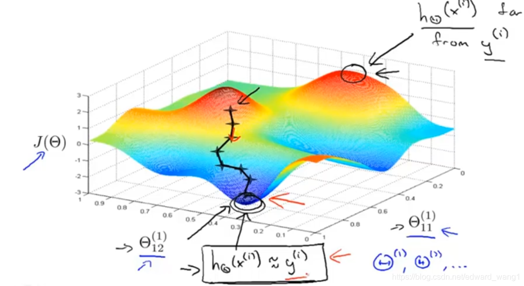
This was actually similar to the figure that I was using earlier to explain gradient descent. So,we have some cost function, and we have a number of parameters in our neural network. Here I've just written down two of the parameter values. In reality, of course, in the neural network, we can have lots of parameters like these. $\Theta ^{(1)}$ , $\Theta ^{(2)}$ all of these are of matrices. So we can have very high dimensional parameters. But because of the limitations of the source of parts we can draw, I'm pretending that we have only two parameters in this neural network. Although obviously we have a lot more in practice. Now, this cost function of $J(\Theta )$ measures how well the neural network fits the training data. So, if you take a point like this one, down here (bottom-left black circle), that's a point where $J(\Theta )$ is pretty low, and so this corresponds to a setting of the parameters. There's a setting of the parameters theta where for most of the training examples, the output of my hyhothesis $h_{\theta }(x^{(i)})$ , that may be pretty close to $y^{(i)}$ . And if this is true, then that's what causes my cost function to be pretty low. Whereas in contrast, if you were to take a value like that (top-right black circle), a point of that corresponds to, where for many training examples, the output of my neural network $h_{\theta }(x^{(i)})$ is far from the actual value $y^{(i)}$ that was observed in the training set. So points like this on the right correspond to where the hypothesis, where the neural network is outputting values on the training set that are far from $y^{(i)}$ . So, it's not fitting the training set well, whereas point like this with low values of the cost function corresponds to where $J(\Theta )$ is low, and therefore corresponds to where the neural network happens to be fitting my training set well because I mean this is what's needed to be true in order for $J(\Theta )$ to be small. So what gradient descent does is we'll start from some random initial point like one over there, and it will repeatedly go downhill. And so what back propagation is doing is computing the direction of the gradient, and what gradient descent is doing is it's taking little steps downhill until hopefully it gets to, in this case, a pretty good local optimum. So, when you implement back propagation and use gardient descent or one of the advanced optimization methods, this picture surely explains what the algorithm is doing. It's trying to find a value of the parameters where the output values in the neural network closely matches the values of the $y^{(i)}s$ observed in your training set.

So, hopefully this gives you a better sense of how the many different pieces of neural network learning fit together. In case even after this video, in case you still feel like there are a lot of different pieces and it's not entirely clear what some of them do or how of these pieces come together, that's actually okay. Neural network learning and back propagation is a complicated algorithm. And even though I've seen the math behind back propagation for many years and I've used back propagation, I think very successfully, for many years, even today I still feel like I don't always have a great grasp of exactly what back propagation is doing sometimes. And what the optimization process looks like of minimizing $J(\Theta )$ . This is much harder algorithm to feel like I have a much less good handle on exactly what this is doing compare to say, linear regression or logistic regression. Which were mathetically and conceptually much simpler and much cleaner algorithms. But so in case you feel the same way, you know, that's actually perfectly ok. But if you do implement back propagation, hopefully what you find is that this is one of the most powerful learning algorithm and if you implement this algorithm, implement back propagation, implement one of these optimization methods, you'll find that back propagation will be able to fit very complex, powerfull, non-linear functions to your data, and this is one of the most effective learning algorithms we have today.

<end>