Qimera Patch Test

---

---

How to Start

• Patch Test option from Tools menu of Main Menu bar

What it Does

The Qimera patch test tool allows for calibration of the angular offsets of either the multibeam or motion sensor system as well as the time latency of the position system.  

General Description

Patch test operations are done using the prioritized position and motion system.  If you wish to establish angular offsets or position latency for secondary systems, you must re-prioritize these as the primary sensor for the patch test Raw Sonar Files using the Processing Settings dialog and then run the patch test session again.  This will not overwrite the offsets established for the original primary sensors.

Patch Test Main Application Window

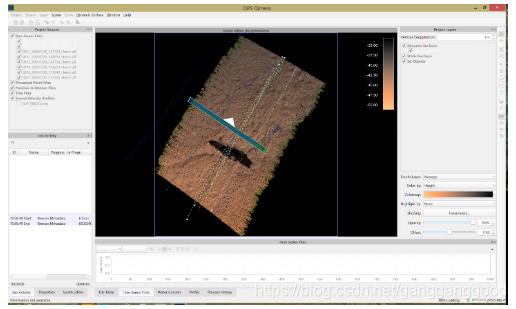
The patch test tool is meant to work in conjunction with the Qimera 4D Scene in the main Qimera application window, this is where the user can choose appropriate spatial subsets of data to examine for the purposes of calibration.  The process begins by selecting 2 or more Raw Sonar Files from the Qimera Project Sources Dock and then accessing Patch Test under the Tools menu.  The Patch Test tool automatically chooses the first two lines of the set and then draws a Dynamic Selection box in the Qimera 4D Scene centered on the average location of the two lines.  Most of the functionality of Qimera is locked down when running the Patch Test tool so it is advisable to set view preferences prior to running the tool, for example, setting the color map to Copper to better highlight the color coding of footprint locations or survey lines in the scene.  Note that some users like to investigate offsets with just a single file, this is possible to do as of Qimera 1.4, but largely nonsensical in terms of a typical patch test procedure.

Patch Test Main Window

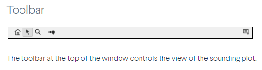
The majority of the user interaction for a patch test calibration is done in the Patch Test main window.  It has 5 main areas as indicated in the Display and Control section below.  A toolbar at the top of the window controls the view of the sounding plot and buttons at the bottom control save and exit of the tool.

Show Rejected

By default, the patch test tool only plots valid soundings.  If you want to see all soundings, including rejected ones, then enable this option.

Save Patch Plot to Image

Saves the patch test plot area to an image file (JPEG or PNG).

Save RMS Plot to Image

Saves the RMS plot area to an image file (JPEG or PNG).

Show Grid Lines

Show/Hide the grid lines in your plot surfaces.

Apply Multibeam Offsets to Both TX and RX

This is an advanced option that will force the multibeam system patch test offsets to be applied to both the transmitter and receiver. This only affects multibeam systems whose transmitter and receiver are at different locations (for example, deep water multibeam systems). This option is auto-detected and checked for systems with the transmitter and receiver at the same location.

If this box is unchecked, and you decide not to apply the offsets to both the transmitter and receiver, Qimera will apply the multibeam offsets as follows:

1. Sounding Plot:  The sounding plot shows the footprint solutions for the spatial subset chosen in the Qimera 4D Scene for the subset of lines that are currently selected from the Lines list (3).  Depth is on the y-axis and distance on the x-axis.  The distance on the x-axis is along the long axis of the spatial selection box from the 4D Scene with zero being the center point along the long axis of the box.

2. Selection Sets:  Qimera will attempt to build a list of all possible reasonable combination of line pairings for any particular patch test calibration parameter.  For example, a good candidate pair for a roll offset determination would be a pair of lines that run in opposite directions (reciprocal heading) and roughly the same speed over roughly the same patch of seafloor.  All possible pairings are examined for all possible offset types (roll, pitch, heading and positioning latency) and those that meet predefined criteria are listed in the Selection Sets list.  You can then choose any pairing from this list; three things will then happen:
   1. The Lines list selection will be updated to use the two candidate lines.
   2. The offset type will update in the Offset combo box in the Current Calibration area (4).  The slider bar will be set to 0.0 and the RMS plot will reset.
   3. The Qimera 4D Scene spatial selection box will be updated to the center position of the two lines with a size and orientation that is appropriate for the type of offset being solved.  For example, solving for a roll offset requires a long thin box whose long axis is oriented orthogonal to the vessel track lines.  Qimera does not take the seafloor topography into account so the user must position the spatial selection box appropriately over a suitable target area.  The Dynamic Selection box can be rotated, re-positioned and re-sized via mouse action on the box.  Mouse roll-over hint icons will indicate which actions are possible based on the location of the mouse cursor in or on the box.
3. Lines: If the set of calibration lines provides reasonable auto-pairing selection sets, you will rarely have to use the Lines dialog.  In the event that the auto-pairing failed, you can still select lines in manual mode (this will be the only item in the Selection Sets list available) by selecting lines in the Lines list.  One or more lines can be selected.  Additionally, if you choose one of the auto-paired Selection Sets items, you can still add/remove lines from the selection using the Lines list window.
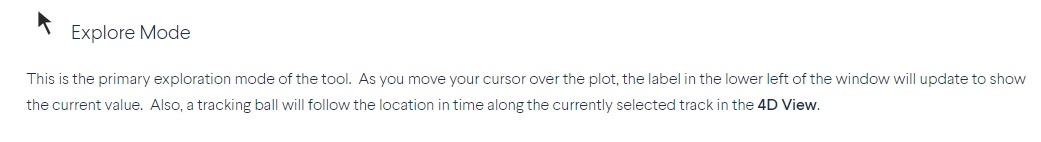
4. Current Calibration: Once lines are selected, you can adjust the calibration parameter of interest.  As you adjust a parameter of interest using the slider bar, the Sounding Plot and the RMS Plot will both update.  The slider bar is adjusted until the soundings from all of the selected lines report consistent results.  Alternately, the auto-solve function can be run.  Once a suitable result is achieved, the value is added to the Cumulative Offsets (5).  This tool is explained in more detail below in the next section.
5. Cumulative Offsets: The patch test tool can be used in an iterative manner, for example the roll, pitch and heading offsets can be roughly determined in a first pass and then improved in a second pass.  With this type of workflow, it is important to allow for the accumulation of offsets through the process.  As you determine offsets and then incrementally improve them, the total of all offsets are shown in this section of the tool.
6. RMS Plot: This is a plot of the root-mean-square (RMS) difference between two temporary terrain models derived from the the two currently selected lines (one terrain model for each line, stored only in memory).  It will update when running the auto-solve function and also when manually adjusting the slider and spin box widgets in the Current Calibration widget set.  This plot is explained in more detail below in the next section.

7. Current Calibration

   The image below highlights the controls and the numbered list below the image explains how each is used.

8. 

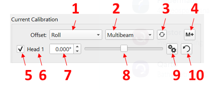
• Offset type combo box: The type of offset being resolved is chosen from this combo box.  The choices are roll, pitch, heading and latency.
• System selection combo box: The angular offsets as resolved by a patch test can either be attributed to either the multibeam or the motion sensor.  This combo box allows you to choose which system you would like to assign the offsets to.  In some cases, you may have multibeam sonar offsets that were accurately measured by a marine surveyor and you may want to resolve the unknown angular offsets of the motion sensor.  In other cases, the motion sensor is well aligned and you may want to assign the patch test results to the multibeam heads.
• Auto solve: This launches the auto-solve routine.  This is described in more detail in the RMS Plot section below.
•   Add calibration: Once you are satisfied with the calibration, the value can be added to the cumulative offsets, these are shown in the Cumulative Offsets section.
• Application: this toggles whether or not this calibration value is enabled or disabled.  This is useful for quickly examining before/after scenarios, particularly for screen shots documenting your calibration.
• Sensor label: this indicates the name of the sensor you are calibrating.
• Offset adjustment spin box: You can enter the offset in the spin box or adjust it using the adjustment arrows that are part of the spin box controller.
• Offset adjustment slider bar: You can adjust the offset using this slider bar.  Holding down the shift key decreases the sensitivity to mouse movement so that small adjustments can be made to fine tune an offset.
•    Range edit: Adjust the minimum and maximum range of the slider bar.  The default is to limit this to +/-5 degrees.
•   Reset zero: Resets the current offset value to zero.  The cumulative offset achieved at this point retains its current value.

• RMS Plot

  Your eye is amazingly adept at subjectively assessing the quality of the chosen calibration offset by looking at the Sounding Plot alone.  It is often desirable, however, to have a quantitative assessment of the quality of the chosen calibration value relative to the entire range of possible calibration values.  The RMS plot allows you to assess the quality of the calibration in a quantitative way by computing the RMS between two temporary terrain models, one for each of the two currently selected survey lines.  This value is computed every time a manual adjustment is made to the Offset Adjustment spinbox and/or slider bar, or when triggering the auto-solve function.  The temporary terrain models, which are stored only in memory, are built for the area associated with the spatial selection box.  The resolution of the temporary terrain models is determined automatically based on the sounding density in the selected area.

  The RMS plot, shown below, has a few graphical components that warrant more explanation. The RMS plot also has a small toolbar at the top that allows for basic view control of the graph with a zoom out button, explore button and zoom button that function in the same manner as they do in the Sounding Plot. The numbered list below provides information about the plot and widget items shown in the RMS plot.

• RMS value for a particular offset, plotted as red dots, either from the auto-solve or from manual adjustments to the Offset adjustment spinbox and/or slider bar widgets. The number and spacing of plotted points depends on whether they are derived from manual adjustments or from the auto-solve function:
  1. The auto-solve function will compute the RMS values over the range of values associated with the Current Calibration slider bar widget limits (which is adjusted by the Range Edit button). The range is split into ten intervals. A large range in the slider bar widget will necessarilly have a large step size in the auto-solve. Decreasing the range of the slider bar widget will decrease the step size taken during the auto-solve.
  2. Manual adjustment of the slider bar or spinbox widgets in the Current Calibration will dynamically fill in the RMS plot with more points. The update rate of the plot will depend on the speed of your computer and its ability to keep up with your adjustments. This allows you to fill in the gaps between the steps taken by the auto-solve algorithm. Recall that holding down the shift key decreases the sensitivity to mouse movement so that small adjustments can be made to fine tune an offset.
• Parabolic fit to the RMS values computed during the auto-solve, as determined via the method of Least Squares. All auto-solve actions attempt to fit a parabola, regardless of the shape traced out by the RMS points.
• Minimum point on the parabola fit to the auto-solve results. The x-value in the graph associated with the parabola minimum is the result from the auto-solve. If the parabola fit is very poor, then the auto-solve does not provide the minimum point as a solution and a warning dialog is shown to indicate that perhaps another set of lines or another spatial selection might yield a better result.
• Text display of the offset and RMS associated with the mouse position in the graph, this updates with mouse motion over the plot.

•  

  

• Buttons

  Save and Apply

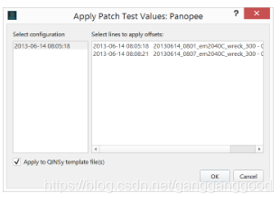
  This button allows you to save a copy of your patch test results to a file which can then be applied to the vessel configuration files associated with all raw sonar files from the same vessel.  You will be presented with a file selection dialog in which you choose a file path and provide a file name.  This file name will be used to save a patch test session file and also a patch test report file (in .pdf format).  Afterward, you will be presented with a dialog (shown below) which allows you to choose which raw sonar files you would like to apply the patch test results to.  Clicking in the right hand list allows you to perform a standard multiselection.  Qimera stores the total offsets in the patch test results, i.e. the value prior to the patch test with the patch test offset applied.  For example, if your initial roll offset was 0.1 deg and your patch test evaluation came up with an additional 0.05 deg, the patch test result file will store the sum of these, i.e. 0.15 deg.  When a patch test session file is applied to an existing vessel configuration, the offsets overwrite the values in the vessel configuration to avoid the pitfalls of accidental double application in the case where the offsets are added.  For files that are imported at a later stage, you must apply the patch test configuration to the newly imported files as discussed in the Qimera Vessel Editor documentation.

  There is an additional option in this dialog that is enabled for QINSy users who work with QINSy .db files.  You can choose to save the patch test results back to a Template.db file to enable quick turnaround to get straight back to mapping.  By enabling the "Apply to QINSy template file(s)" checkbox, Qimera will isolate the directories in which the raw .db files came from and will search the directories for template.db files.  For each template.db file found in the search directories, Qimera will examine the MBE systems in the template.db file and will only write out the patch test offsets for the systems that match those that were in the raw .db files that were provided to the Patch Test tool. This prevents writing offsets to another template file which may have a different MBE system in it.

• 

• Save a Copy

  Saving a copy does the same as 'Save and Apply' except there is no application step.  The patch test session file and report will be saved in the directory that you choose from the file selection dialog.

  Exit

  This button exits the tool without saving any results or reports.

  Dual Head

  If you are patch testing a dual headed system, you can evaluate the offsets in the same patch test session.  An additional view control button will be displayed in the toolbar that lets you toggle the visibility of the port and starboard heads in the sounding plot.

    Display both heads

    Display port head only

    Display starboard head only

  

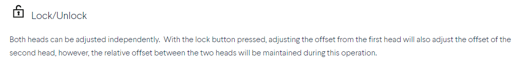
•  A second set of control widgets will appear in the Current Calibration that allows for separate control of the 2nd head.  A second set of cumulative offsets will also be shown in the Cumulative Offsets area.  A lock button also appears in the Current Calibration that allows the slider values to lock relative to each other such that you can establish common offsets shared by both heads, e.g. if the MRU is misaligned, both heads will appear to share a common roll offset but they will also have a residual offset relative to each other.

•