Deeplab图像语义分割网络-学习笔记

备注：本文源于一篇外文文献 此文档是我的学习翻译版，看原文应点击链接。

Deeplab Image Semantic Segmentation Network

Deeplab图像语义分割网络

Jan 29, 2018

   

Introduction

Deep Convolution Neural Networks (DCNNs) have achieved remarkable success in various Computer Vision applications. Like others, the task of semantic segmentation is not an exception to this trend.

深度卷积神经网络（DCNN）在各种计算机视觉应用中取得了显着的成功。 与其他人一样，语义分割的任务也不是这种趋势的例外。

This piece provides an introduction to Semantic Segmentation with a hands-on TensorFlow implementation. We go over one of the most relevant papers on Semantic Segmentation of general objects - Deeplab_v3. You can clone the notebook for this post here.

本文通过实际操作TensorFlow实现了语义分段的介绍。 我们回顾了一篇关于一般对象语义分割的最相关的论文 - Deeplab_v3。 您可以在此处克隆此帖子的笔记。

Semantic Segmentation 语义分割

Regular image classification DCNNs have similar structure. These models take images as input and output a single value representing the category of that image.

常规图像分类DCNN具有相似的结构。 这些模型将图像作为输入并输出表示该图像类别的单个值。

Usually, classification DCNNs have four main operations. Convolutions, activation function, pooling, and fully-connected layers. Passing an image through a series of these operations outputs a feature vector containing the probabilities for each class label. Note that in this setup, we categorize an image as a whole. That is, we assign a single label to an entire image.

通常，分类DCNN有四个主要操作。 卷积，激活功能，池化和完全连接的层。 通过一系列这些操作传递图像输出包含每个类标签的概率的特征向量。 请注意，在此设置中，我们将图像整体分类。 也就是说，我们为整个图像分配一个标签。

Standard deep learning model for image recognition.

用于图像识别的标准深度学习模型。

Image credits: Convolutional Neural Network MathWorks.
图片来源：卷积神经网络MathWorks。

Different from image classification, in semantic segmentation we want to make decisions for every pixel in an image. So, for each pixel, the model needs to classify it as one of the pre-determined classes. Put another way, semantic segmentation means understanding images at a pixel level.

与图像分类不同，在语义分割中，我们希望为图像中的每个像素做出决策。 因此，对于每个像素，模型需要将其分类为预定类之一。 换句话说，语义分割意味着在像素级别理解图像。

Keep in mind that semantic segmentation doesn’t differentiate between object instances. Here, we try to assign an individual label to each pixel of a digital image. Thus, if we have two objects of the same class, they end up having the same category label. Instance Segmentation is the class of problems that differentiate instances of the same class.

请记住，语义分段不区分对象实例。 在这里，我们尝试为数字图像的每个像素分配单独的标签。 因此，如果我们有两个相同类的对象，它们最终会有相同的类别标签。 实例分段是区分同一类实例的一类问题。

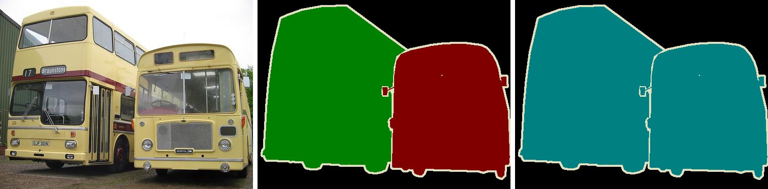
Difference between Semantic Segmentation and Instance Segmentation. (middle) Although they are the same object (bus) they are classified as different objects. (left) Same object, equal category.

语义分割与实例分割的区别。 （中）虽然它们是同一个对象（总线），但它们被归类为不同的对象。 （左）相同的对象，相同的类别。

Yet, regular DCNNs such as the AlexNet and VGG aren’t suitable for dense prediction tasks. First, these models contain many layers designed to reduce the spatial dimensions of the input features. As a consequence, these layers end up producing highly decimated feature vectors that lack sharp details. Second, fully-connected layers have fixed sizes and loose spatial information during computation.

然而，诸如AlexNet和VGG的常规DCNN不适合于密集预测任务。 首先，这些模型包含许多层，旨在减少输入要素的空间维度。 因此，这些层最终会产生缺乏清晰细节的高度抽取的特征向量。 其次，完全连接的层在计算期间具有固定的大小和松散的空间信息。

As an example, instead of having pooling and fully-connected layers, imagine passing an image through a series of convolutions. We can set each convolution to have stride of 1 and “SAME” padding. Doing this, each convolution preserves the spatial dimensions of its input. We can stack a bunch of these convolutions and have a segmentation model.

作为一个例子，想象一下通过一系列卷积传递图像，而不是拥有池和完全连接的层。 我们可以将每个卷积设置为1和“SAME”填充。 这样做，每个卷积保留其输入的空间维度。 我们可以堆叠一堆这些卷积并具有分段模型。

Fully-Convolution neural network for dense prediction task. Note the non-existence of pooling and fully-connected layers.

This model could output a probability tensor with shape [W,H,C], where W and H represent the Width and Height. And C the number of class labels. Applying the argmax function (on the third axis) gives us a tensor shape of [W,H,1]. After, we compute the cross-entropy loss between each pixel of the ground-truth images and our predictions. In the end, we average that value and train the network using back prop.

用于密集预测任务的全卷积神经网络。 注意池和完全连接的层不存在。
该模型可以输出具有形状[W，H，C]的概率张量，其中W和H表示宽度和高度。 和C类标签的数量。 应用argmax函数（在第三轴上）给出了[W，H，1]的张量形状。 之后，我们计算地面实况图像的每个像素与我们的预测之间的交叉熵损失。 最后，我们平均该值并使用后支柱训练网络。

There is one problem with this approach though. As we mentioned, using convolutions with stride 1 and “SAME” padding preserves the input dimensions. However, doing that would make the model super expensive in both ways. Memory consumption and computation complexity.

但是这种方法存在一个问题。 正如我们所提到的，使用带有步幅1和“SAME”填充的卷积可以保留输入尺寸。 但是，这样做会使模型在两个方面都非常昂贵。 内存消耗和计算复杂性。

To ease that problem, segmentation networks usually have three main components. Convolutions, downsampling, and upsampling layers.

为了解决这个问题，分段网络通常有三个主要组件。 卷积，下采样和上采样层。

Encoder-decoder architecture for Image Semantic Segmentation.

There are two common ways to do downsampling in neural nets. By using convolution striding or regular pooling operations. In general, downsampling has one goal. To reduce the spatial dimensions of given feature maps. For that reason, downsampling allows us to perform deeper convolutions without much memory concerns. Yet, they do it in detriment of losing some features in the process.

用于图像语义分割的编码器 - 解码器架构。
在神经网络中进行下采样有两种常用方法。 通过使用卷积跨越或常规池操作。 通常，下采样有一个目标。 减少给定要素图的空间维度。 出于这个原因，下采样允许我们在没有太多内存问题的情况下执行更深层次的卷积。 然而，他们这样做不利于在此过程中失去一些功能。

Also, note that the first part of this architecture looks a lot like usual classification DCNNs. With one exception, they do not put in place fully-connected layers.

另请注意，此体系结构的第一部分看起来很像通常的分类DCNN。 除了一个例外，它们不会建立完全连接的层。

After the first part, we have a feature vector with shape [w,h,d] where w, h and d are the width, height and depth of the feature tensor. Note that the spatial dimensions of this compressed vector are smaller (yet denser) than the original input.

在第一部分之后，我们有一个形状为[w，h，d]的特征向量，其中w，h和d是特征张量的宽度，高度和深度。 请注意，此压缩矢量的空间维度比原始输入更小（但更密集）。

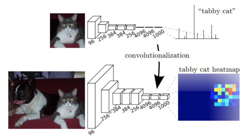
(Top) VGG-16 network on its original form. Note the 3 fully-connected layers on top of the convolution stack. (Down) VGG-16 model when substituting its fully-connected layers to 1x1 convolutions. This change allows the network to output a coarse heat-map.

（顶部）VGG-16网络的原始形式。 注意卷积堆栈顶部的3个完全连接的层。 （下）VGG-16模型在将其全连接层替换为1x1卷积时。 此更改允许网络输出粗略的热图

Image credits: Fully Convolutional Networks for Semantic Segmentation.

At this point, regular classification DCNNs would output a dense (non-spatial) vector containing probabilities for each class label. Instead, we feed this compressed feature vector to a series of upsampling layers. These layers work on reconstructing the output of the first part of the network. The goal is to increase the spatial resolution so the output vector has the same dimensions as the input.

此时，常规分类DCNN将输出包含每个类标签的概率的密集（非空间）向量。 相反，我们将此压缩特征向量提供给一系列上采样层。 这些层用于重建网络第一部分的输出。 目标是增加空间分辨率，使输出矢量具有与输入相同的尺寸。

Usually, upsampling layers are based on strided transpose convolutions. These functions go from deep and narrow layers to wider and shallower ones. Here, we use transpose convolutions to increase feature vectors dimension to the desired value.

通常，上采样层基于跨步的转置卷积。 这些功能从深层和窄层变为更宽更浅的层。 在这里，我们使用转置卷积将特征向量维度增加到所需的值。

In most papers, these two components of a segmentation network are called: encoder and decoder. In short, the first, “encodes” its information into a compressed vector used to represent its input. The second (the decoder) works on reconstructing this signal to the desired outcome.

在大多数论文中，分段网络的这两个组件称为：编码器和解码器。 简而言之，第一个，将其信息“编码”为用于表示其输入的压缩矢量。 第二个（解码器）致力于将该信号重建为期望的结果。

There are many network implementations based on encoder-decoder architectures. FCNs, SegNetand UNet are some of the most popular ones. As a result, we have seen many successful segmentation models in a variety of fields.

存在许多基于编码器 - 解码器架构的网络实现。 FCN，SegNet和UNet是最受欢迎的一些。 因此，我们在各个领域都看到了许多成功的细分模型。

Model Architecture 模型架构

Different from most encoder-decoder designs, Deeplab offers a different approach to semantic segmentation. It presents an architecture for controlling signal decimation and learning multi-scale contextual features.
与大多数编码器 - 解码器设计不同，Deeplab提供了一种不同的语义分割方法。 它提出了一种用于控制信号抽取和学习多尺度上下文特征的架构。

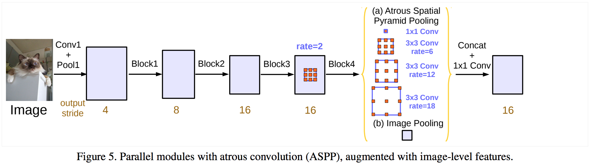
Image credits: Rethinking Atrous Convolution for Semantic Image Segmentation.

Deeplab uses an ImageNet pre-trained ResNet as its main feature extractor network. However, it proposes a new Residual block for multi-scale feature learning. Instead of regular convolutions, the last ResNet block uses atrous convolutions. Also, each convolution (within this new block) uses different dilation rates to capture multi-scale context.

Deeplab使用ImageNet预训练的ResNet作为其主要特征提取器网络。 但是，它提出了一种用于多尺度特征学习的新残差块。 最后一个ResNet块不使用常规卷积，而是使用有害卷积。 此外，每个卷积（在此新块内）使用不同的扩张率来捕获多尺度上下文。

Additionally, on top of this new block, it uses Atrous Spatial Pyramid Pooling (ASPP). ASPP uses dilated convolutions with different rates as an attempt of classifying regions of an arbitrary scale.

此外，在这个新块的顶部，它使用了Atrous Spatial Pyramid Pooling（ASPP）。 ASPP使用具有不同速率的扩张卷积作为对任意尺度的区域进行分类的尝试。

To understand the deeplab architecture, we need to focus on three components. (i) The ResNet architecture, (ii) atrous convolutions and (iii) Atrous Spatial Pyramid Pooling (ASPP). Let’s go over each one of them.

要了解deeplab架构，我们需要关注三个组件。 （i）ResNet架构，（ii）痛苦的卷积和（iii）Atrous空间金字塔池（ASPP）。 让我们来看看他们中的每一个。

ResNets

ResNet is a very popular DCNN that won the ILSVRC 2015 classification task. One of the main contributions of ResNets was to provide a framework to ease the training of deeper models.

ResNet是一个非常受欢迎的DCNN，赢得了ILSVRC 2015分类任务。 ResNets的主要贡献之一是提供一个框架来简化深层模型的培训。

In its original form, ResNets contain 4 computational blocks. Each block contains a different number of Residual Units. These units perform a series of convolutions in a special way. Also, each block is intercalated with max-pooling operations to reduce spatial dimensions.

在其原始形式中，ResNets包含4个计算块。 每个块包含不同数量的剩余单元。 这些单元以特殊方式执行一系列卷积。 此外，每个块都插入了最大池操作以减少空间维度。

The original paper presents two types of Residual Units. The baseline and the bottleneck blocks.

在其原始形式中，ResNets包含4个计算块。 每个块包含不同数量的剩余单元。 这些单元以特殊方式执行一系列卷积。 此外，每个块都插入了最大池操作以减少空间维度。

The baseline unit contains two 3x3 convolutions with Batch Normalization(BN) and ReLU activations.

原始论文提出了两种类型的剩余单位。 基线和瓶颈块。基线单元包含两个3x3卷积，具有批量标准化（BN）和ReLU激活。
 

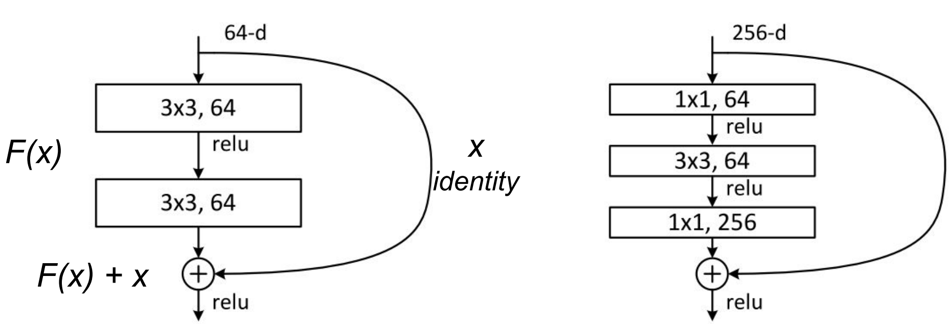
ResNet building blocks. (left) baseline; (right) bottleneck unit

Adapted from: Deep Residual Learning for Image Recognition.

The second, the bottleneck unit, consists of three stacked operations. A series of 1x1, 3x3 and 1x1convolutions substitute the previous design. The two 1x1 operations are designed for reducing and restoring dimensions. This leaves the 3x3 convolution, in the middle, to operate on a less dense feature vector. Also, BN is applied after each convolution and before ReLU non-linearity.

第二个是瓶颈单元，由三个堆叠操作组成。一系列1x1,3x3和1x1转换代替了之前的设计。这两个1x1操作旨在减少和恢复尺寸。这使得中间的3x3卷积在较不密集的特征向量上运行。此外，在每个卷积之后和ReLU非线性之前应用BN。

To help to understand, let’s denote these group of operations as a function F of its input x.

为了帮助理解，让我们将这些操作组表示为其输入x的函数F.

After the non-linear transformations in F(x), the unit combines the result of F(x) with the original input x. This combination is done by adding the two functions. Merging the original input x with the non-linear function F(x) offers some advantages. It allows earlier layers to access the gradient signal from later layers. In other words, skipping the operations on F(x) allows earlier layers to have access to a stronger gradient signal. As a result, this type of connectivity has been shown to ease the training of deeper networks.

在F（x）中的非线性变换之后，该单元将F（x）的结果与原始输入x组合。通过添加两个函数来完成此组合。将原始输入x与非线性函数F（x）合并提供了一些优点。它允许较早的层访问后面的层的梯度信号。换句话说，跳过F（x）上的操作允许较早的层能够访问更强的梯度信号。因此，这种类型的连接已被证明可以简化对更深层网络的培训。

Non-bottleneck units also show gain in accuracy as we increase model capacity. Yet, bottleneck residual units have some practical advantages. First, it performs more computations having almost the same number of parameters. Second, they also perform in a similar computational complexity as its counterpart.

随着我们增加模型容量，非瓶颈单元也显示出准确性的提高。然而，瓶颈残留单元具有一些实际优势。首先，它执行具有几乎相同数量的参数的更多计算。其次，它们的执行速度与其对应的计算复杂度相似。

In practice, bottleneck units are more suitable for training deeper models because of less training time and computational resources need.

在实践中，由于较少的训练时间和计算资源需求，瓶颈单元更适合训练更深的模型。

For our implementation, we use the full pre-activation Residual Unit. The only difference, from the standard bottleneck unit, lies in the order in which BN and ReLU activations are placed. For the full pre-activation, BN and ReLU (in this order) occur before convolutions.

对于我们的实施，我们使用完整的预激活残留单元。 与标准瓶颈单元的唯一区别在于BN和ReLU激活的顺序。 对于完全预激活，BN和ReLU（按此顺序）在卷积之前发生。

Different ResNet building block architectures. (Left-most) the original ResNet block. (Right-most) the improved full pre-activation version.

Image credits: Identity Mappings in Deep Residual Networks.

As shown in Identity Mappings in Deep Residual Networks, the full pre-activation unit performs better than other variants.

如深度残留网络中的身份映射所示，完整的预激活单元比其他变体表现更好。

Note that the only difference between these designs is the order of BN and RELu in the convolution stack.

请注意，这些设计之间的唯一区别是卷积堆栈中BN和RELu的顺序。

Atrous Convolutions

Atrous (or dilated) convolutions are regular convolutions with a factor that allows us to expand the filter’s field of view.

Atrous（或扩张）卷积是常规卷积，其中一个因子允许我们扩展滤波器的视野。

Consider a 3x3 convolution filter for instance. When the dilation rate is equal to 1, it behaves like a standard convolution. But, if we set the dilation factor to 2, it has the effect of enlarging the convolution kernel.

例如，考虑一个3x3卷积滤波器。 当扩张率等于1时，它表现得像标准卷积。 但是，如果我们将扩张系数设置为2，它会产生扩大卷积核的效果。

In theory, it works like that. First, it expands (dilates) the convolution filter according to the dilation rate. Second, it fills the empty spaces with zeros - creating a sparse like filter. Finally, it performs regular convolution using the dilated filter.

从理论上讲，它就是这样的。 首先，它根据膨胀率扩展（扩张）卷积滤波器。 其次，它用零填充空白空间 - 创建稀疏的过滤器。 最后，它使用扩张的滤波器执行常规卷积。

Atrous convolutions with various rates.  各种费率的萎缩卷积。

As a consequence, a convolution with a dilated 2, 3x3 filter would make it able to cover an area equivalent to a 5x5. Yet, because it acts like a sparse filter, only the original 3x3 cells will do computation and produce results. I said “act” because most frameworks don’t implement atrous convolutions using sparse filters - because of memory concerns.

因此，使用扩张的2,3x3滤波器进行卷积将使其能够覆盖相当于5x5的面积。 然而，因为它的作用类似于稀疏滤波器，所以只有原始的3x3单元才能进行计算并产生结果。 我之所以说“行为”是因为大多数框架都没有使用稀疏过滤器来实现有害卷积 - 因为内存问题。

In a similar way, setting the atrous factor to 3 allows a regular 3x3 convolution to get signals from a 7x7 corresponding area.

以类似的方式，将atrous因子设置为3允许常规的3x3卷积从7x7对应区域获取信号。

This effect allows us to control the resolution at which we compute feature responses. Also, atrous convolution adds larger context without increasing the number of parameters or the amount of computation.

Deeplab also shows that the dilation rate must be tuned according to the size of the feature maps. They studied the consequences of using large dilation rates over small feature maps.

此效果允许我们控制计算特征响应的分辨率。 此外，萎缩卷积在不增加参数数量或计算量的情况下增加了更大的上下文。

Deeplab还表明，必须根据要素图的大小调整扩张率。 他们研究了在小特征图上使用大的扩张率的后果。

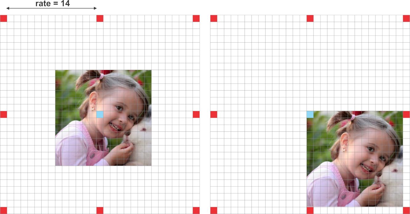
Side effects of setting larger dilation rates for smaller feature maps. For a 14x14 input image, a *3x3* filter with dilation rate of 15 makes the atrous convolution behaves like a regular 1x1 convolution.

为较小的特征图设置较大的扩张率的副作用。 对于14x14输入图像，扩散率为15的* 3x3 *滤波器使得迂回卷积的行为类似于常规的1x1卷积。

When the dilation rate is very close to the feature map’s size, a regular 3x3 atrous filter acts as a standard 1x1 convolution.

当扩张速率非常接近特征图的大小时，常规的3x3 atrous滤波器充当标准的1x1卷积。

Put in another way, the efficiency of atrous convolutions depends on a good choice of the dilation rate. Because of that, it is important to know the concept of output stride in neural networks.

换句话说，萎缩卷曲的效率取决于扩张率的良好选择。 因此，了解神经网络中输出步幅的概念非常重要。

Output stride explains the ratio of the input image size to the output feature map size. It defines how much signal decimation the input vector suffers as it passes the network.

输出步幅解释了输入图像大小与输出要素图大小的比率。它定义了输入向量在通过网络时遭受的信号抽取量。

For an output stride of 16, an image size of 224x224x3 outputs a feature vector with 16 times smaller dimensions. That is 14x14.

对于16的输出步幅，224x224x3的图像尺寸输出尺寸小16倍的特征向量。那是14x14。

Besides, Deeplab also debates the effects of different output strides on segmentation models. It argues that excessive signal decimation is harmful for dense prediction tasks. In short, models with smaller output stride - less signal decimation - tends to output finer segmentation results. Yet, training models with smaller output stride demand more training time.

此外，Deeplab还讨论了不同输出步幅对分割模型的影响。它认为过度的信号抽取对密集预测任务是有害的。简而言之，具有较小输出步幅的模型 - 较少的信号抽取 - 倾向于输出更精细的分割结果。然而，具有较小输出的训练模型需要更多的训练时间。Deeplab reports experiments with two configurations of output strides, 8 and 16. As expected, output stride = 8 was able to produce slightly better results. Here we choose output stride = 16 for practical reasons.

Deeplab报告了两种输出步幅配置的实验，8和16.正如预期的那样，输出stride = 8能够产生稍好的结果。这里我们选择输出stride = 16出于实际原因。

Also, because the atrous block doesn’t implement downsampling, ASPP also runs on the same feature response size. As a result, it allows learning features from multi-scale context using relative large dilation rates.

此外，由于atrous块没有实现下采样，ASPP也运行相同的功能响应大小。因此，它允许使用相对大的扩张率从多尺度背景学习特征。

The new Atrous Residual Block contains three residual units. In total, the 3 units have three 3x3convolutions. Motivated by multigrid methods, Deeplab proposes different dilation rates for each convolution. In summary, multigrid defines the dilation rates for each of the three convolutions.

新的Atrous残余块包含三个剩余单元。总共有3个单位有3个3x3对话。在多重网格方法的推动下，Deeplab为每个卷积提出了不同的扩张率。总之，多重网格定义了三个卷积中每个卷积的扩张率。
 

In practice:

For the new block4, when output stride = 16 and Multi Grid = (1, 2, 4), the three convolutions have rates = 2 · (1, 2, 4) = (2, 4, 8) respectively.

对于新的block4，当输出stride = 16且Multi Grid =（1,2,4）时，三个回旋分别具有速率= 2·（1,2,4）=（2,4,8）。

Atrous Spatial Pyramid Pooling

For ASPP, the idea is to provide the model with multi-scale information. To do that, ASPP adds a series atrous convolutions with different dilation rates. These rates are designed to capture long-range context. Also, to add global context information, ASPP incorporates image-level features via Global Average Pooling (GAP).

对于ASPP，其想法是为模型提供多尺度信息。为此，ASPP增加了一系列不同的扩张率的萎缩卷积。这些费率旨在捕捉长期背景。此外，为了添加全局上下文信息，ASPP通过全局平均池（GAP）合并了图像级功能。

This version of ASPP contains 4 parallel operations. These are a 1x1 convolution and three 3x3convolutions with dilation rates =(6,12,18). As we mentioned, at this point, the feature maps’ nominal stride is equal to 16.

此版本的ASPP包含4个并行操作。这些是1x1卷积和3个3x3对称，扩张率=（6,12,18）。正如我们所提到的，此时，特征图的标称步幅等于16。

Based on the original implementation, we use crop sizes of 513x513 for both: training and testing. Thus, using an output stride 16 means that ASPP receives feature vectors of size 32x32.

根据最初的实施，我们使用513x513的裁剪尺寸：训练和测试。因此，使用输出步幅16意味着ASPP接收大小为32×32的特征向量。Also, to add more global context information, ASPP incorporates image-level features. First, it applies GAP to the output features from the last atrous block. Second, the resulting features are fed to a 1x1 convolution with 256 filters. Finally, the result is bilinearly upsampled to the correct dimensions.

此外，为了添加更多全局上下文信息，ASPP包含图像级功能。首先，它将GAP应用于最后一个块的输出特征。其次，将得到的特征馈送到具有256个滤波器的1x1卷积。最后，结果以双线性上采样到正确的尺寸。

@slim.add_arg_scope
def atrous_spatial_pyramid_pooling(net, scope, depth=256):
    """
    ASPP consists of (a) one 1×1 convolution and three 3×3 convolutions with rates = (6, 12, 18) when output stride = 16
    (all with 256 filters and batch normalization), and (b) the image-level features as described in https://arxiv.org/abs/1706.05587
    :param net: tensor of shape [BATCH_SIZE, WIDTH, HEIGHT, DEPTH]
    :param scope: scope name of the aspp layer
    :return: network layer with aspp applyed to it.
    """

    with tf.variable_scope(scope):
        feature_map_size = tf.shape(net)

        # apply global average pooling
        image_level_features = tf.reduce_mean(net, [1, 2], name='image_level_global_pool', keep_dims=True)
        image_level_features = slim.conv2d(image_level_features, depth, [1, 1], scope="image_level_conv_1x1", activation_fn=None)
        image_level_features = tf.image.resize_bilinear(image_level_features, (feature_map_size[1], feature_map_size[2]))

        at_pool1x1 = slim.conv2d(net, depth, [1, 1], scope="conv_1x1_0", activation_fn=None)

        at_pool3x3_1 = slim.conv2d(net, depth, [3, 3], scope="conv_3x3_1", rate=6, activation_fn=None)

        at_pool3x3_2 = slim.conv2d(net, depth, [3, 3], scope="conv_3x3_2", rate=12, activation_fn=None)

        at_pool3x3_3 = slim.conv2d(net, depth, [3, 3], scope="conv_3x3_3", rate=18, activation_fn=None)

        net = tf.concat((image_level_features, at_pool1x1, at_pool3x3_1, at_pool3x3_2, at_pool3x3_3), axis=3,
                        name="concat")
        net = slim.conv2d(net, depth, [1, 1], scope="conv_1x1_output", activation_fn=None)
        return net

In the end, the features, from all the branches, are combined into a single vector via concatenation. This output is then convoluted with another 1x1 kernel - using BN and 256 filters.

最后，来自所有分支的特征通过连接组合成单个向量。 然后使用BN和256个过滤器将此输出与另一个1x1内核进行卷积。

After ASPP, we feed the result to another 1x1 convolution - to produce the final segmentation logits.

在ASPP之后，我们将结果提供给另一个1x1卷积 - 以产生最终的分段logits。

Implementation Details

Using the ResNet-50 as feature extractor, this implementation of Deeplab_v3 employs the following network configuration:

使用ResNet-50作为特征提取器，Deeplab_v3的这种实现采用以下网络配置：

• output stride = 16     输出stride = 16
• Fixed multi-grid atrous convolution rates of (1,2,4) to the new Atrous Residual block (block 4).   
• 修复了（1,2,4）新的Atrous残余块的多网格迂回卷积率（方框4）。
• ASPP with rates (6,12,18) after the last Atrous Residual block.
• ASPP在最后一次Atrous Residual块之后的费率（6,12,18）。

Setting output stride to 16 gives us the advantage of substantially faster training. Comparing to output stride of 8, stride of 16 makes the Atrous Residual block deals with 4 times smaller feature maps than its counterpart.

将输出步幅设置为16使我们获得了大大加快训练的优势。与8的输出步幅相比，16的步幅使得Atrous Residual块处理的特征映射比其对应的要小4倍。

The multi-grid dilation rates are applied to the 3 convolutions inside the Atrous Residual block.

多网格膨胀率应用于Atrous残余块内的3个卷积。

Finally, each of the three parallel 3x3 convolutions in ASPP gets a different dilation rate - (6,12,18).

最后，ASPP中三个平行的3x3卷积中的每一个都得到不同的扩张率 - （6,12,18）。

Before computing the cross-entropy error, we resize the logits to the input’s size. As argued in the paper, it’s better to resize the logits than the ground-truth labels to keep resolution details.

在计算交叉熵错误之前，我们将logits的大小调整为输入的大小。正如论文中所论述的那样，最好调整logits的大小而不是地面实况标签以保持分辨率细节。

Based on the original training procedures, we scale each image using a random factor from 0.5 to 2. Also, we apply random left-right flipping to the scaled images.

基于原始训练程序，我们使用从0.5到2的随机因子来缩放每个图像。此外，我们将随机左右翻转应用于缩放图像。

Finally, we crop patches of size 513x513 for both training and testing.

最后，我们为训练和测试修剪了大小为513x513的补丁

def deeplab_v3(inputs, args, is_training, reuse):

    # mean subtraction normalization
    inputs = inputs - [_R_MEAN, _G_MEAN, _B_MEAN]

    # inputs has shape [batch, 513, 513, 3]
    with slim.arg_scope(resnet_utils.resnet_arg_scope(args.l2_regularizer, is_training,
                                                      args.batch_norm_decay,
                                                      args.batch_norm_epsilon)):
        resnet = getattr(resnet_v2, args.resnet_model) # get one of the resnet models: resnet_v2_50, resnet_v2_101 ...
        _, end_points = resnet(inputs,
                               args.number_of_classes,
                               is_training=is_training,
                               global_pool=False,
                               spatial_squeeze=False,
                               output_stride=args.output_stride,
                               reuse=reuse)

        with tf.variable_scope("DeepLab_v3", reuse=reuse):

            # get block 4 feature outputs
            net = end_points[args.resnet_model + '/block4']

            net = atrous_spatial_pyramid_pooling(net, "ASPP_layer", depth=256, reuse=reuse)

            net = slim.conv2d(net, args.number_of_classes, [1, 1], activation_fn=None,
                              normalizer_fn=None, scope='logits')

            size = tf.shape(inputs)[1:3]
            # resize the output logits to match the labels dimensions
            #net = tf.image.resize_nearest_neighbor(net, size)
            net = tf.image.resize_bilinear(net, size)
            return net

To implement atrous convolutions with multi-grid in the block4 of the resnet, we just changed this piece in the resnet_utils.py file.

为了在resnet的block4中使用多网格实现有害的卷积，我们只是在resnet_utils.py文件中更改了这个部分。

...
with tf.variable_scope('unit_%d' % (i + 1), values=[net]):
  # If we have reached the target output_stride, then we need to employ
  # atrous convolution with stride=1 and multiply the atrous rate by the
  # current unit's stride for use in subsequent layers.
  if output_stride is not None and current_stride == output_stride:
    # Only uses atrous convolutions with multi-graid rates in the last (block4) block
    if block.scope == "block4":
      net = block.unit_fn(net, rate=rate * multi_grid[i], **dict(unit, stride=1))
    else:
      net = block.unit_fn(net, rate=rate, **dict(unit, stride=1))
    rate *= unit.get('stride', 1)
...

Training

To train the network, we decided to use the augmented Pascal VOC dataset provided by Semantic contours from inverse detectors. 为了训练网络，我们决定使用来自反向探测器的语义轮廓提供的增强Pascal VOC数据集。

The training data is composed of 8,252 images. 5,623 from the training set and 2,299 from the validation set. To test the model using the original VOC 2012 val dataset, I removed 558 images from the 2,299 validation set. These 558 samples were also present on the official VOC validation set. Also, I added 330 images from the VOC 2012 train set that weren’t present either among the 5,623 nor the 2,299 sets. Finally, 10% of the 8,252 images (~825 samples) are held for validation, leaving the rest for training.

训练数据由8,252幅图像组成。 来自训练集的5,623和来自验证集的2,299。 为了使用原始VOC 2012 val数据集测试模型，我从2,299验证集中删除了558个图像。 这些558个样品也出现在官方VOC验证集上。 此外，我还添加了来自VOC 2012火车组的330张图像，这些图像在5,623和2,299套中都不存在。 最后，8,252张图像中的10％（约825个样本）被保留用于验证，剩下的用于训练。

Note that different from the original paper, this implementation is not pre-trained in the COCO dataset. Also, some of the techniques described in the paper for training and evaluation were not queried out.

请注意，与原始论文不同，此实现未在COCO数据集中预先训练。 此外，还没有查询文章中描述的用于培训和评估的一些技术。

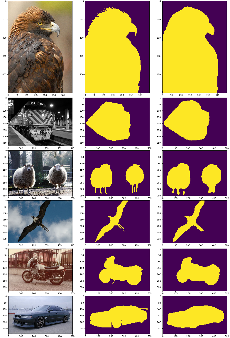
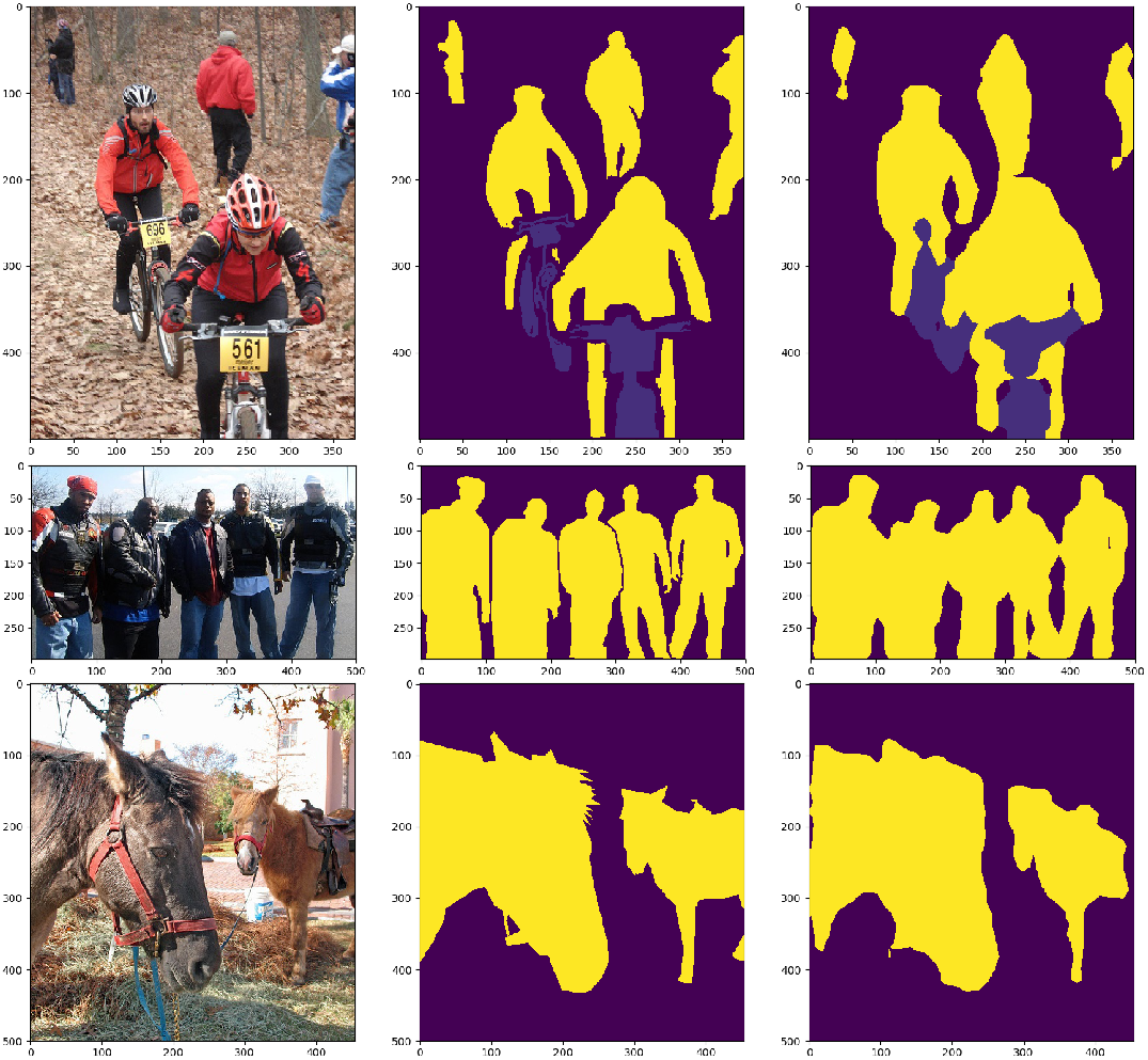
Results

The model was able to achieve decent results on the PASCAL VOC validation set.

• Pixel accuracy: ~91%
• Mean Accuracy: ~82%
• Mean Intersection over Union (mIoU): ~74%
• Frequency weighed Intersection over Union: ~86%.

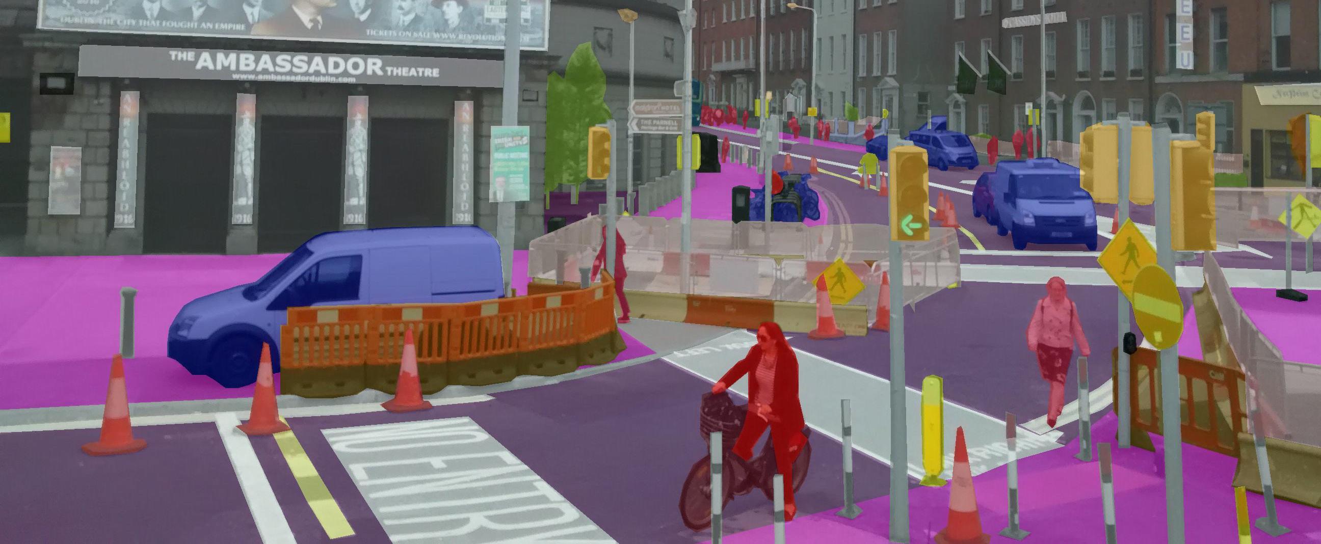
Bellow, you can check out some of the results in a variety of images from the PASCAL VOC validation set.

Concluding

The field of Semantic Segmentation is no doubt one of the hottest ones in Computer Vision. Deeplab presents an alternative to classic encoder-decoder architectures. It advocates the usage of atrous convolutions for feature learning in multi-range contexts. Feel free to clone the repo and tune the model to achieve closer results to the original implementation. The complete code is here.

Hope you like reading!