SIFT: Theory and Practice - Finding keypoints（转）

SIFT: Theory and Practice

 

---

Finding keypoints

Series: SIFT: Theory and Practice:

1. Introduction
2. The scale space
3. LoG approximations
4. Finding keypoints
5. Getting rid of low contrast keypoints
6. Keypoint orientations
7. Generating a feature

Up till now, we have generated a scale space and used the scale space to calculate the Difference of Gaussians. Those are then used to calculate Laplacian of Gaussian approximations that is scale invariant. I told you that they produce great key points. Here's how it's done!

Finding key points is a two part process

1. Locate maxima/minima in DoG images
2. Find subpixel maxima/minima

Locate maxima/minima in DoG images

The first step is to coarsely locate the maxima and minima. This is simple. You iterate through each pixel and check all it's neighbours. The check is done within the current image, and also the one above and below it. Something like this:

X marks the current pixel. The green circles mark the neighbours. This way, a total of 26 checks are made. X is marked as a "key point" if it is the greatest or least of all 26 neighbours.

Usually, a non-maxima or non-minima position won't have to go through all 26 checks. A few initial checks will usually sufficient to discard it.

Note that keypoints are not detected in the lowermost and topmost scales. There simply aren't enough neighbours to do the comparison. So simply skip them!

Once this is done, the marked points are the approximate maxima and minima. They are "approximate" because the maxima/minima almost never lies exactly on a pixel. It lies somewhere between the pixel. But we simply cannot access data "between" pixels. So, we must mathematically locate the subpixel location.

Here's what I mean:

The red crosses mark pixels in the image. But the actual extreme point is the green one.

Find subpixel maxima/minima

Using the available pixel data, subpixel values are generated. This is done by the Taylor expansion of the image around the approximate key point.

Mathematically, it's like this:

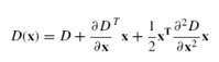
We can easily find the extreme points of this equation (differentiate and equate to zero). On solving, we'll get subpixel key point locations. These subpixel values increase chances of matching and stability of the algorithm.

Example

Here's a result I got from the example image I've been using till now:

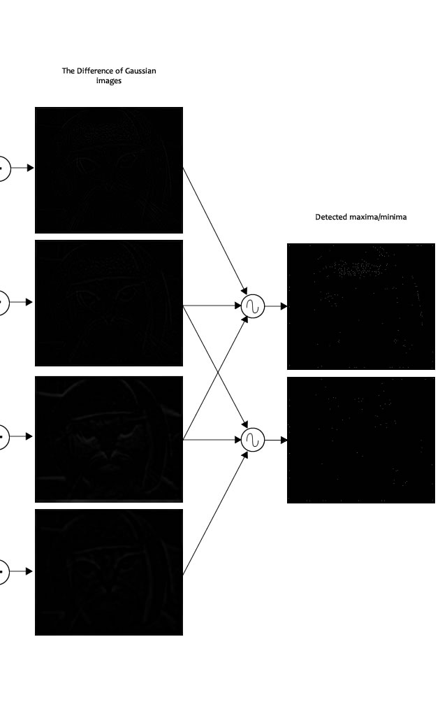
The maxima detector. Trust me, there are a bunch of white dots on those black images. The compressions / etc got in the way.

The author of SIFT recommends generating two such extrema images. So, you need exactly 4 DoG images. To generate 4 DoG images, you need 5 Gaussian blurred images. Hence the 5 level of blurs in each octave.

In the image, I've shown just one octave. This is done for all octaves. Also, this image just shows the first part of keypoint detection. The Taylor series part has been skipped.

Summary

Here, we detected the maxima and minima in the DoG images generated in the previous step. This is done by comparing neighbouring pixels in the current scale, the scale "above" and the scale "below".

Next, we'll reject some keypoints detected here. This is because they either don't have enough contrast or they lie on an edge

---

More in the series

This tutorial is part of a series called SIFT: Theory and Practice:

1. Introduction
2. The scale space
3. LoG approximations
4. Finding keypoints
5. Getting rid of low contrast keypoints
6. Keypoint orientations
7. Generating a feature