机器学习（三），使用tensorflow进行线性回归--建模

前言

茴字有13种写法其实才是深入学习的有效方式

上一篇文章使用 tensorflow 初步 完成了线性回归，继续尝试使用建模的方式优化代码，并将训练的结果保存了下来。

题目

考虑一个实际问题，某城市在 2013 年 - 2018 年的房价如下表所示：

年份	2013	2014	2015	2016	2017	2018
房价	12000	14000	15000	16500	17500	18400

现在，我们希望通过对该数据进行线性回归，即使用线性模型 y = ax + b 来拟合上述数据，此处 a 和 b 是待求的参数。

环境

开发环境比较简单，安装 最新 anaconda 即可， 我安装的版本默认内置 python 3.8。 使用Spyder 执行代码， spyder默认不能跑plt 图像界面，前往 修改设置即可。

打开 Anaconda Prompt 命令行，安装 tensorflow

pip install -i https://pypi.tuna.tsinghua.edu.cn/simple tensorflow

分析

优化代码的目的是去掉一些自行撰写的部分，使用tensorflow 内置的模块来替代。

• 损失函数 更换为

 losses = tf.losses.MeanSquaredError()
 loss = losses(y_pred, y)  # 传入 推导的值，标签值
 loss = tf.reduce_mean(loss)  # 求和

• 梯度的计算 更换为

with tf.GradientTape() as tape:
grads = tape.gradient(loss, model.variables)    # 使用 model.variables 这一属性直接获得模型中的所有变量

• 优化器 更换为

# 优化器 随机梯度下降法(SGD)
optimizer = tf.keras.optimizers.SGD(learning_rate=5e-4)
optimizer.apply_gradients(grads_and_vars=zip(grads, model.variables))

完整的训练源码如下：

# -*- coding: utf-8 -*-
"""
Created on Sun Feb 21 21:04:10 2021

@author: huwp001

Dependencies:
tensorflow: 2.0
matplotlib
numpy

使用 tensorflow 建立模型 进行梯度下降训练。 
"""

import os
os.environ["CUDA_DEVICE_ORDER"] = "PCI_BUS_ID"  
os.environ["CUDA_VISIBLE_DEVICES"] = "-1"

import tensorflow as tf
import numpy as np
import matplotlib.pyplot as plt

"""
原始数据 X_raw, y_raw
"""
X_raw = np.array([2013, 2014, 2015, 2016, 2017, 2018], dtype=np.float32)
y_raw = np.array([12000, 14000, 15000, 16500, 17500, 18400], dtype=np.float32)

"""
进行归一化，转换为了 0,1 之间的值
"""
X = (X_raw - X_raw.min()) / (X_raw.max() - X_raw.min())
y = (y_raw - y_raw.min()) / (y_raw.max() - y_raw.min())

X = X.reshape(-1,1)
y = y.reshape(-1,1)

X = tf.constant(X)
y = tf.constant(y)

# 定义模型
class MyLinear(tf.keras.Model):
    def __init__(self):
        super().__init__()
        self.dense = tf.keras.layers.Dense(
            units=1,
            activation=None,
            kernel_initializer=tf.zeros_initializer(),
            bias_initializer=tf.zeros_initializer()
        )

    def call(self, input):
        output = self.dense(input)
        return output
 
model = MyLinear()
num_epoch = 20000
# 优化器 随机梯度下降法(SGD)
optimizer = tf.keras.optimizers.SGD(learning_rate=5e-4)
# loss 函数：MSE
losses = tf.losses.MeanSquaredError()

for e in range(num_epoch):
    with tf.GradientTape() as tape:
        y_pred = model(X)      # 调用模型 y_pred = model(X) 而不是显式写出 y_pred = a * X + b
        loss = losses(y_pred, y)
        loss = tf.reduce_mean(loss)
    grads = tape.gradient(loss, model.variables)    # 使用 model.variables 这一属性直接获得模型中的所有变量
    optimizer.apply_gradients(grads_and_vars=zip(grads, model.variables))
    if e % 50 == 0 or e==num_epoch-1:
        plt.cla()
        plt.scatter(X, y)
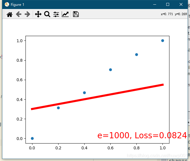
        plt.plot(X, y_pred, 'r-', lw=5)
        plt.text(0.5, 0, 'e=%d, Loss=%.4f' % (e, loss), fontdict={'size': 20, 'color': 'red'})
        plt.pause(0.1)
        
# 保存训练得到的参数
model.save_weights('model3.weight')

为方便展示，使用plt模块增加了推导进度的显示，可以看到 我们从一个 横线 y=0*x+0， 推导得到 最终的结果。

运行

执行程序开始推导，红线是初始 y=ax+b， 且 a=b=0， 由于使用了model，暂时获取不到 a，b ，这个待研究。

循环20000次后结果，红线比较完美的穿过数据点。感觉学习的效率比上两篇差。自己写函数可能效率还是高一些。

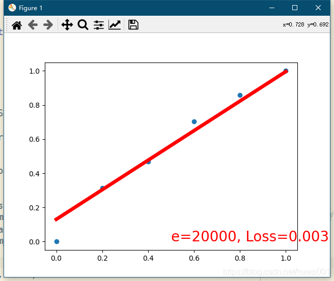
训练的结果保存了下来，然后下一步我们进行模型评估。

模型评估代码如下：

# -*- coding: utf-8 -*-
"""
Created on Mon Feb 22 17:49:28 2021

@author: Administrator

Dependencies:
tensorflow: 2.0
matplotlib
numpy

读取训练好的模型，进行模型评估

""" 

import tensorflow as tf
import numpy as np
import matplotlib.pyplot as plt

"""
原始数据 X_raw, y_raw
"""
X_raw = np.array([2013, 2014, 2015, 2016, 2017, 2018], dtype=np.float32)
y_raw = np.array([12000, 14000, 15000, 16500, 17500, 18400], dtype=np.float32)


X2_raw = np.array([2019, 2020], dtype=np.float32)

"""
进行归一化，转换为了 0,1 之间的值
"""
X = (X_raw - X_raw.min()) / (X_raw.max() - X_raw.min())
y = (y_raw - y_raw.min()) / (y_raw.max() - y_raw.min())

X = X.reshape(-1,1)
y = y.reshape(-1,1)

X = tf.constant(X)
y = tf.constant(y)

X2 = (X2_raw - X_raw.min()) / (X_raw.max() - X_raw.min())
X2 = X2.reshape(-1,1)
X2 = tf.constant(X2)

class MyLinear(tf.keras.Model):
    def __init__(self):
        super().__init__()
        self.dense = tf.keras.layers.Dense(
            units=1,
            activation=None,
            kernel_initializer=tf.zeros_initializer(),
            bias_initializer=tf.zeros_initializer()
        )

    def call(self, input):
        output = self.dense(input)
        return output
    
model = MyLinear()
model.load_weights('model3.weight')

# 先对原始数据进行 回归验证
y_pred = model.predict(X)
metrics_f = tf.keras.metrics.mean_squared_error(y, y_pred)
loss = tf.reduce_sum(metrics_f);
print("test accuracy: " , loss)

# 对 新数据进行预测
y_pred2 = model.predict(X2)

plt.cla()
plt.scatter(X, y)
plt.plot(X, y_pred, 'r-', lw=5)
plt.scatter(X2, y_pred2)
plt.plot(X2, y_pred2, 'r-', lw=5)
plt.text(0.5, 0, 'Accuracy=%.4f' % (loss), fontdict={'size': 20, 'color': 'red'})

运行代码，得到如图：

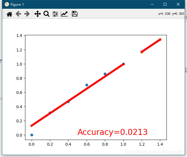
注意我这里先读取模型，再次验证了原始数据，然后对新数据X2 进行预测，展示如图。预测的结果从图像上还是可信的。

总结

和上一篇相比，使用了Model，完全隐藏了 手动计算梯度等过程，函数表达式也看不到了，好在结果基本一致。

下一篇继续就一元一次函数学习 tensorflow 的写法。

参考文章：

简单粗暴 tensorflow2 前往